17  Seasonal and Panel Data Models

17.1 Introduction

Following on from our review of ARIMA models, we’ll complete our section on time series analysis by exploring seasonal and panel-data models. These models are useful when dealing with data that exhibits regular patterns over time, or data that spans multiple entities across various time periods.

Seasonal models specifically help in understanding and forecasting periodic fluctuations that occur at regular intervals, such as quarterly sales cycles or annual temperature variations. They adjust for seasonal effects to provide a clearer insight into underlying trends and cycles that might be obscured by these periodic changes.

Panel-data models, on the other hand, are used when data involves observations over multiple time periods for the same entities, such as individuals, companies, or countries.

17.2 Seasonal Time Series Analysis

17.2.1 Introduction

Seasonal time series analysis deals with patterns that repeat at regular intervals, such as monthly sales peaks or weekly energy consumption cycles. In earlier reading, we encountered fundamental concepts like stationarity, trend, and autocorrelation. Seasonal analysis extends these ideas by focusing on regular, calendar-based fluctuations.

Recognising seasonality is crucial for accurate forecasts because ignoring recurring patterns often leads to systematic errors. A simple example is when winter-related sales show predictable spikes year after year. Understanding these cycles can aid in resource allocation and inventory planning.

Contemporary methods make it relatively easy to spot and measure seasonal effects, but it remains vital to check if the pattern truly repeats each cycle. Some series appear seasonal, but are actually influenced by sporadic events or longer-term trends that ‘masquerade’ as seasonality.

17.2.2 Identifying seasonal patterns using decomposition

Traditional decomposition methods, covered in an earlier chapter, break a time series into trend, seasonal, and residual components. By plotting these components, we can visually confirm if a seasonal pattern is present and consistent over time.

Note that this technique builds on the idea that different processes, like growth over years (trend) and monthly oscillations (seasonal), can be separated.

Classical decomposition is often based on averages over fixed intervals, such as calculating monthly means to detect annual seasonal effects. Each data point is then compared to the overall mean for that month, revealing a persistent up-or-down shift.

After decomposition, the seasonal component provides a clear view of how each period deviates from the average. This helps not only in forecasting but also in explaining why certain months or quarters perform better or worse than expected.

Example

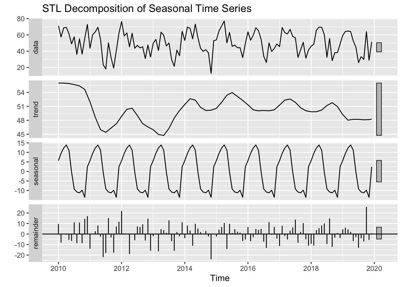
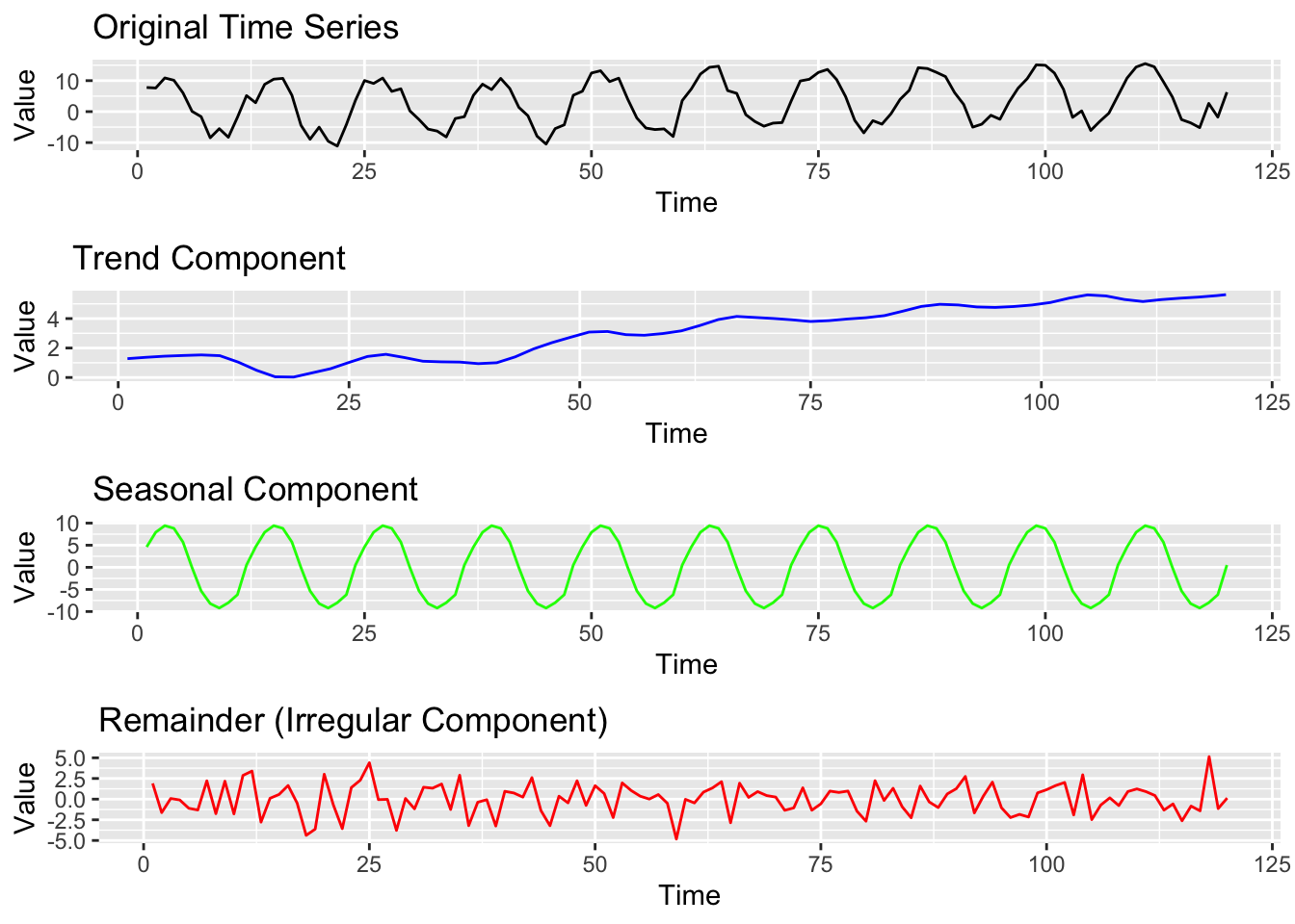
The figure above shows the decomposition of a seasonal time series into its three main components: trend, seasonality, and residual (random noise).

Decomposition helps us analyse the underlying structure of a time series by isolating these elements. The trend represents the long-term movement, the seasonal component captures recurring patterns, and the residual represents the remaining fluctuations that cannot be explained by trend or seasonality.

17.2.3 Seasonal indices and adjustments

Seasonal indices measure how much a period deviates from the baseline. A monthly index of 1.2, for instance, means values for that month are typically 20% above average. These indices are derived through decomposition or by averaging deviations across similar time points.

By using seasonal indices, we can adjust data to remove cyclical effects, highlighting long-term trends. This ensures fair comparisons across months or quarters by eliminating predictable seasonal peaks or dips.

For example, in football, goal-scoring rates may be higher in the early season and dip during winter. Seasonal adjustment allows analysts to compare player performance more accurately by accounting for these fluctuations.

Seasonal indices thus serve a dual purpose: they reveal underlying trends by removing repeating cycles and improve forecasting by allowing seasonality to be applied or removed as needed.

Example

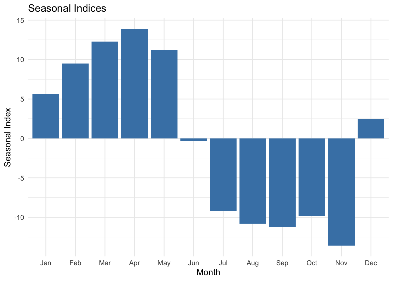
Seasonal indices measure the extent to which each season (e.g., month) deviates from the overall mean of the time series. The bar chart below displays the average seasonal indices for each month, highlighting periods of higher or lower-than-average values. This visualisation is useful for seasonal adjustment, where we remove seasonal fluctuations to better analyse trends.

17.2.4 Seasonal differencing for stationary series

Differencing is a technique we have encountered in previous ARIMA discussions. When a series exhibits strong seasonality, seasonal differencing subtracts the value from the same season in the previous cycle. This step can transform a non-stationary series into a stationary one by removing the repeated patterns over the seasonal period.

For instance, if data are recorded monthly, a seasonal difference might involve subtracting the observation from 12 months ago. This captures and neutralises the annual cycle, making the residual process more stable. In many series, combining seasonal differencing with standard differencing (for trend) is required before applying more advanced models.

While seasonal differencing can be powerful, it is also essential not to over-difference. We should remember that too many differencing steps can strip away meaningful information or introduce artificial patterns into the residuals, undermining the predictive accuracy of the model.

Example

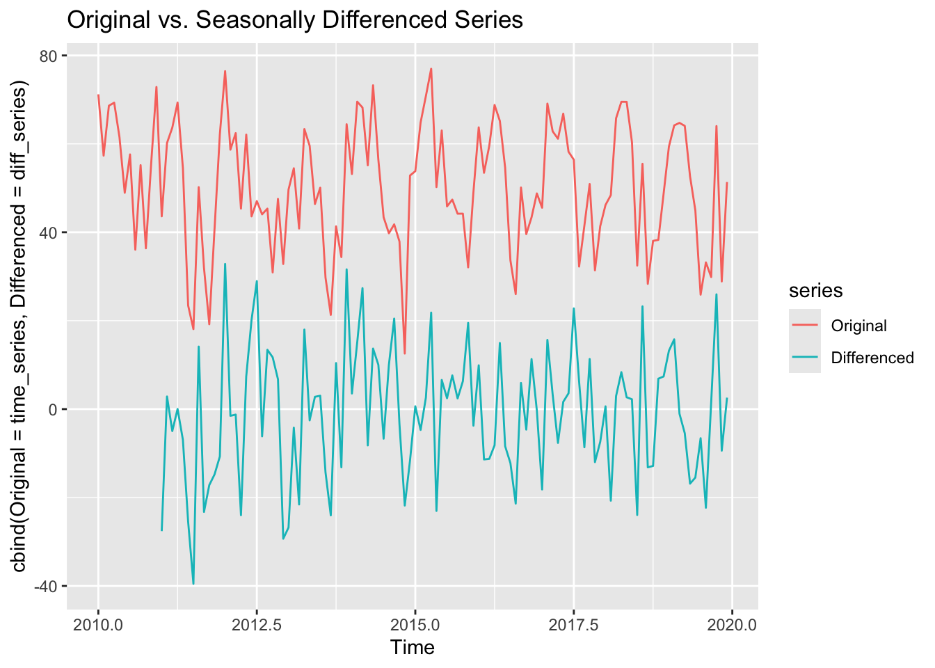
To make a seasonal time series stationary, we apply seasonal differencing. The plot above compares the original series with its seasonally differenced version, where differences between values lagged by one year are taken. This transformation removes seasonal patterns, making the series more suitable for modeling.

17.3 Seasonal Decomposition of Time Series (STL)

17.3.1 Introduction

STL (Seasonal and Trend decomposition using Loess) is a more flexible approach than classical decomposition. It uses robust local regression to separate a time series into trend, seasonal, and remainder components. This method is adaptive, meaning it can handle changing patterns in both the trend and the magnitude of seasonality.

Compared to traditional techniques, STL offers better control over how fast the seasonal component can change, which is important for real-world data where seasonal patterns may evolve over time.

Because STL uses iterative smoothing, it can manage anomalies, outliers, or abrupt shifts in the series without completely distorting the extracted seasonal component. However, its flexibility also means there are more tuning parameters, which we must handle with care.

17.3.2 Additive vs. multiplicative decomposition

Decomposition can be additive or multiplicative, reflecting how seasonal effects combine with trend and random fluctuations.

In an additive model, the series is represented as a sum of these components: \(y_t​=Trend_t​+Seasonal_t​+Residual_t\). This is usually suitable when variations around the trend do not grow with the level of the series.

A multiplicative model assumes \(y_t=Trend_t×Seasonal_t×Residualty_t\). This works better when seasonal fluctuations increase as the overall level of the data rises, such as a business whose seasonal sales peaks grow proportionally with its general sales trend.

STL can handle both additive and multiplicative forms, often by transforming data (for instance, using logs) to convert multiplicative dynamics into additive ones. Choosing the correct framework for decomposition ensures we accurately capture how seasonal movements scale over time.

Example

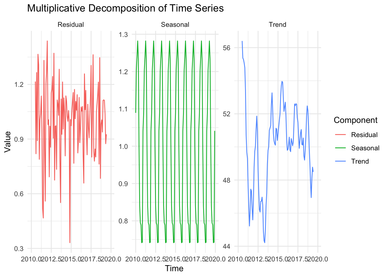
This figure shows multiplicative decomposition. Whiel additive decomposition assumes that the seasonal fluctuations remain constant over time, multiplicative decomposition assumes they scale with the level of the series. If the variation increases as the series grows, a multiplicative model is preferable.

17.3.3 Trend, seasonal, and residual components

Within STL, the trend is derived through repeated smoothing, allowing it to adapt to gradual changes yet remain stable enough to reflect the general direction of the data.

The seasonal component is extracted by focusing on cyclical patterns of a fixed period, but STL’s algorithms allow for slight variations in the pattern from one cycle to the next.

The residual (or remainder) contains whatever is left after removing the trend and seasonal components. This ideally includes only irregular, unpredictable fluctuations.

By isolating this component, we can quickly check for anomalies or possible model mis-specifications. If strong patterns remain in the residuals, the decomposition might be incomplete or incorrectly configured.

Because STL is iterative, each step refines the extracted trend and seasonality until a stable solution is reached. The process can be computationally more intensive than classical decomposition, but software like R readily handles the computations for typical time series lengths.

17.3.4 Applications of STL in Forecasting

STL proves valuable for forecasting because, once the seasonal and trend components are separately identified, we can project those components forward and then recombine them. By focusing on stable patterns, STL-based forecasts may be more accurate for complex, real-world time series than classical approaches.

Another advantage is that the trend can be modelled using simpler methods (like linear regression), or even more sophisticated techniques, while the seasonal part remains flexible. If the seasonal pattern shifts gradually over time, STL can capture that evolution better than fixed seasonal decomposition methods.

Additionally, STL helps in outlier detection by making the underlying structure clear. If the remainder exhibits large spikes that do not fit the usual seasonal or trend changes, we can investigate external causes, refine our forecasts, or adjust the data if needed.

Example

# Forecasting with STL + ETS
stl_forecast <- forecast(stl_decomp, method = "ets", h = 24)

# Plot forecast
autoplot(stl_forecast) + ggtitle("STL Forecasting with ETS")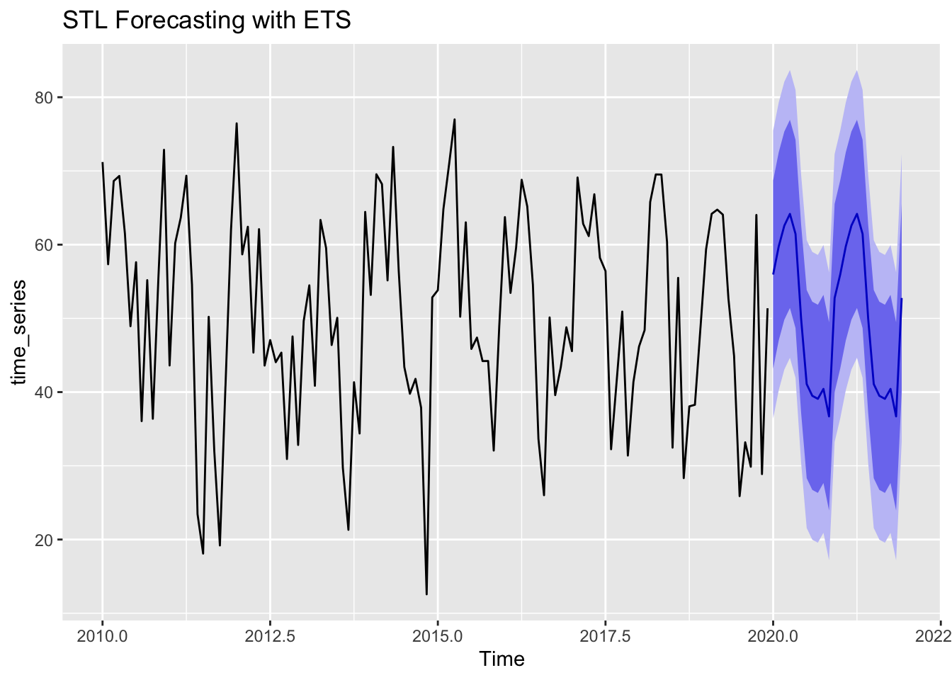

STL decomposition can be combined with exponential smoothing (ETS) to produce accurate forecasts. The forecast plot above shows how the trend and seasonality are used to extend the time series into the future.

17.4 Seasonal ARIMA

17.4.1 Introduction

Seasonal ARIMA, often called SARIMA, extends ARIMA models to handle seasonal patterns. You already know that ARIMA is defined by parameters \((p,d,q)\) for the non-seasonal part. SARIMA adds seasonal terms \((P,D,Q)\) along with a seasonal period \(s\), allowing the model to account for regular repetitions over certain intervals (e.g., monthly data with \(s=12\)).

This extension is particularly useful when a time series exhibits recurring spikes or troughs at fixed intervals, such as holiday-related sales or annual weather cycles. By incorporating the seasonal parameters directly into the ARIMA framework, SARIMA can capture complex correlations.

Despite its added complexity, SARIMA follows the same core principles: differencing is used to achieve stationarity (including seasonal differencing if needed), and the ACF/PACF plots help identify suitable orders for the AR and MA components, both seasonally and non-seasonally.

17.4.2 SARIMA Model Components (p,d,q; P,D,Q)

Like standard ARIMA, \((p,d,q)\) describes the non-seasonal part, where ppp is the order of autoregression, ddd the differencing needed, and qqq the order of moving average. The seasonal components \((P,D,Q)\) mirror this structure but apply at the seasonal lag s. Thus, SARIMA effectively combines two layers of ARIMA: one for short-term dynamics and another for cyclical, seasonal patterns.

For example, a model might be written as: \[ ARIMA(p,d,q) \times (P,D,Q)_s \]

Here, \(D\) indicates how many times seasonal differencing is applied, while \(P\) and \(Q\) capture the autoregressive and moving average terms at multiples of \(s\). Handling these extra parameters can be intricate, but it provides a richer representation for data with strong seasonal repetition.

Choosing SARIMA orders often involves checking seasonal versions of the ACF and PACF. If a spike occurs at lag \(s\), it may suggest a seasonal AR or MA term. Equally, if differencing at lag \(s\) stabilises the series, we know a seasonal differencing component \(D\) is required.

17.4.3 Identifying seasonal lags with ACF and PACF

Previously, we learned to inspect ACF and PACF plots for non-seasonal AR and MA terms. For seasonal data, we also examine correlations at multiples of the seasonal period𝑠. Spikes in the ACF at 𝑠,2𝑠,3𝑠 etc., may indicate a seasonal MA process, while spikes in the PACF at those multiples often suggest a seasonal AR component.

When analysing these plots, it is helpful to distinguish shorter lags (which inform the non-seasonal part) from longer lags that occur at intervals of 𝑠. This distinction aids in deciding whether 𝑃(seasonal AR order) and 𝑄(seasonal MA order) should be nonzero. Moreover, if differencing at lag 𝑠 removes the seasonal pattern, that suggests 𝐷 (seasonal differencing) may be necessary.

Because these plots can become cluttered, analysts often use a combination of:

• Visual inspection
• Formal tests for seasonality
• Automated model selection procedures (e.g., auto.arima with seasonal=TRUE in R)

These methods help guide the selection of appropriate seasonal parameters in ARIMA modeling.

Example

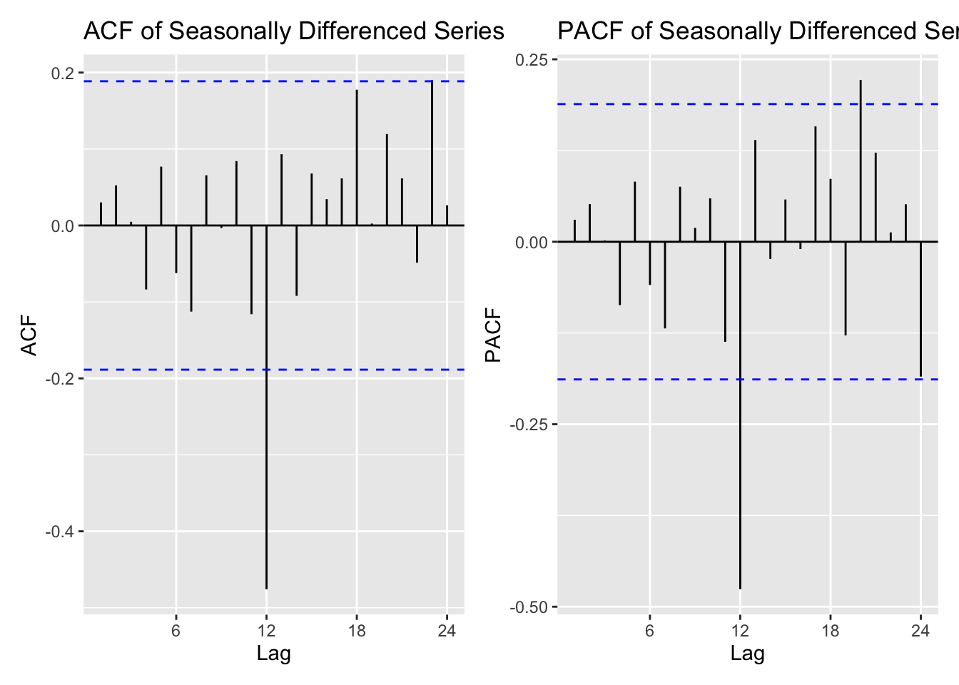
The Autocorrelation function (ACF) and partial autocorrelation function (PACF) plots help identify significant seasonal lags in the data. Peaks at seasonal lags (multiples of 12 months) indicate strong periodic components that should be included in a SARIMA model.

17.4.4 Forecasting with SARIMA Models

Once a SARIMA model is correctly specified, forecasts incorporate both short-term autocorrelations and repeating seasonal cycles. This approach is particularly valuable in fields like retail forecasting, where year-end shopping patterns significantly impact overall predictions.

Always remember to check model diagnostics carefully, ensuring that residuals resemble white noise and that no seasonal spikes remain in the ACF or PACF of the residuals. You should also compare the chosen SARIMA model with non-seasonal ARIMA or simpler seasonal adjustments, balancing complexity against forecast accuracy.

By capturing seasonal dynamics explicitly, SARIMA often outperforms vanilla ARIMA for strongly seasonal data. However, it demands careful attention to parameter selection, stationarity checks, and interpretability, as the added seasonal components increase the risk of overfitting if not handled properly.

Example

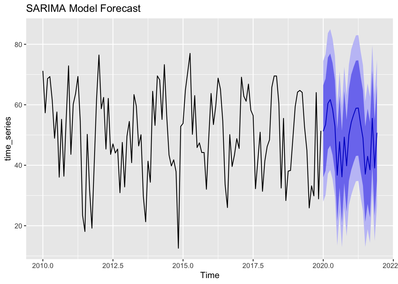
SARIMA (Seasonal ARIMA) is a powerful model for forecasting seasonal time series. The plot above shows a SARIMA-generated forecast, where the model captures both trend and seasonality.

17.5 Panel Data in Time Series

17.5.1 Introduction

Panel data refers to observations of multiple entities, such as individuals, firms, or regions, tracked across time.

It combines the cross-sectional dimension (many entities) with a time series dimension (repeated measurements). This setup can offer important insights into both individual-level changes over time and variations between different entities.

Imagine we collect the following data for 10 football players over 5 seasons (2019–2023). The dataset might include:

Player Performance Data Over Seasons

Player	Season	Goals	Assists	Minutes_Played	Pass_Accuracy
Player A	2019	12	5	2800	82.5
Player A	2020	15	7	2900	84.0
Player A	2021	10	6	2600	80.3
Player B	2019	8	10	2500	78.9
Player B	2020	9	12	2700	80.1
Player C	2019	20	3	3000	88.2

This panel dataset allows us to analyse:

• Trends over time (e.g., does Player A improve each season?).
• Differences between players (e.g., do midfielders have higher pass accuracy than strikers?).
• Impact of external factors (e.g., how does a coaching change affect performance?).

This type of panel data could be useful in forecasting player performance, identifying talent development trends, and analysing the effects of training or tactics over time.

By building on core ARIMA and regression models, panel data allows us to control for unobserved heterogeneity. For instance, two businesses in different locations might have distinct baseline sales levels or cost structures, yet both follow a similar economic cycle. Accounting for these differences yields more accurate and generalisable conclusions.

Because panel data can grow large, computational complexity increases, and model choice becomes more critical. Remember that standard time series techniques might need adjustments to handle multiple cross-sections effectively.

17.5.2 Definition: Cross-sectional data over time

Cross-sectional data snapshots typically capture one moment for many entities, such as a survey of multiple companies in a single month. When these snapshots repeat over multiple periods, we get panel data. This repeated structure allows researchers to see how each entity evolves, while comparing patterns across different entities.

In a time series context, each entity’s history forms its own series, and collectively they form a panel. Hence, not only do we look for trends and seasonality within each series, but we also examine how differences between entities might influence those patterns.

This approach is particularly powerful in economics and social sciences, where we want to track how policy changes or economic shocks affect various groups over time. By contrast, standard single-series analysis might overlook differences between groups or incorrectly attribute cross-sectional effects to time-based trends.

Example

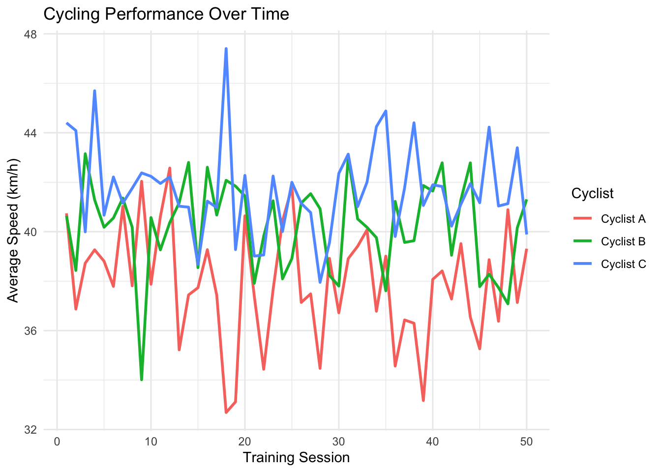
Panel data consists of multiple entities observed over time.

For example, in the figure below each cyclist follows a different performance trend over 50 training sessions.

Notice that Cyclist C consistently records higher average speeds than Cyclist A and B. Speed fluctuations are also captured, showing variation in training performance.

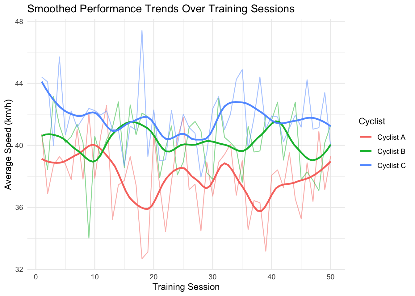
We can apply a LOESS smoothing curve to observe trends in performance over time:

17.5.3 Fixed effects vs. random effects models

When analysts use panel data, they often choose between fixed effects and random effects models.

• Fixed effects models assume that each entity has a unique but constant offset or intercept, capturing individual-specific traits that do not change over time. This method effectively controls for time-invariant factors by differencing them out.

• Random effects models assume these entity-level effects are random variables drawn from a distribution. This approach can be more efficient statistically if the random effect assumption holds true, but it risks bias if the unobserved entity characteristics correlate strongly with the explanatory variables.

In time series contexts, both fixed and random effects can be extended to include lagged variables and autoregressive terms. Keep in mind that the choice between the two often hinges on theoretical considerations and diagnostic tests (like the Hausman test), aiming to ensure consistency and minimal bias.

17.5.4 Applications

Panel data methods apply to a wide variety of problems.

• In finance, analysts can track multiple stocks or firms over time to understand how market conditions affect each company differently.
• In epidemiology, researchers might track patients across multiple clinic visits to see how treatments and demographic variables influence health outcomes over time.

By capturing both within-entity and between-entity variations, panel data offers deeper insights than a single cross-section or a single time series alone.

Note that many standard forecasting techniques, such as ARIMA, can be adapted to panel data by fitting separate models for each entity or building advanced hierarchical structures that borrow information across entities.

While the added complexity can be daunting, modern statistical software and machine learning frameworks provide tools for estimation, prediction, and inference in panel settings.

17.6 Advanced Topics in Time Series Analysis

17.6.1 Introduction

Beyond classical ARIMA, SARIMA, and panel data models, there are advanced techniques that deal with more complex structures and relationships in time series. These methods become essential when data exhibit intricate spatial dependencies, or when multiple time series interact dynamically across large networks.

When you have gained confidence with standard techniques, you might want to explore these advanced methods to tackle specialised forecasting challenges. Although more sophisticated, they build on the same fundamental ideas of stationarity, autocorrelation, and parameter estimation introduced in previous chapters.

Complexity often arises from the need to capture not just the evolution of one series but also the interdependencies between multiple series or multiple locations. Keeping track of these extra connections can greatly improve forecast accuracy and broaden the scope of real-world applications.

17.6.2 Spatio-temporal models

Spatio-temporal models extend time series analysis to account for location-based relationships. In these models, observations are linked across both space and time, meaning that changes in one location can influence neighbouring regions in future periods. Examples include environmental data (pollution levels across cities), agricultural yields in different fields, or real estate prices in multiple neighbourhoods.

Standard approaches might use distance-based weights or neighbourhood structures to capture spatial interactions. These weights can then be integrated into forecasting models that also include time lags, allowing us to forecast a variable’s behaviour in one region based on both its past values and the past values of surrounding areas.

Such models can become quite intricate, requiring advanced mathematics and computational tools. However, they highlight how time series methods can scale beyond one-dimensional temporal data to problems involving multiple dimensions and real-world connectivity.

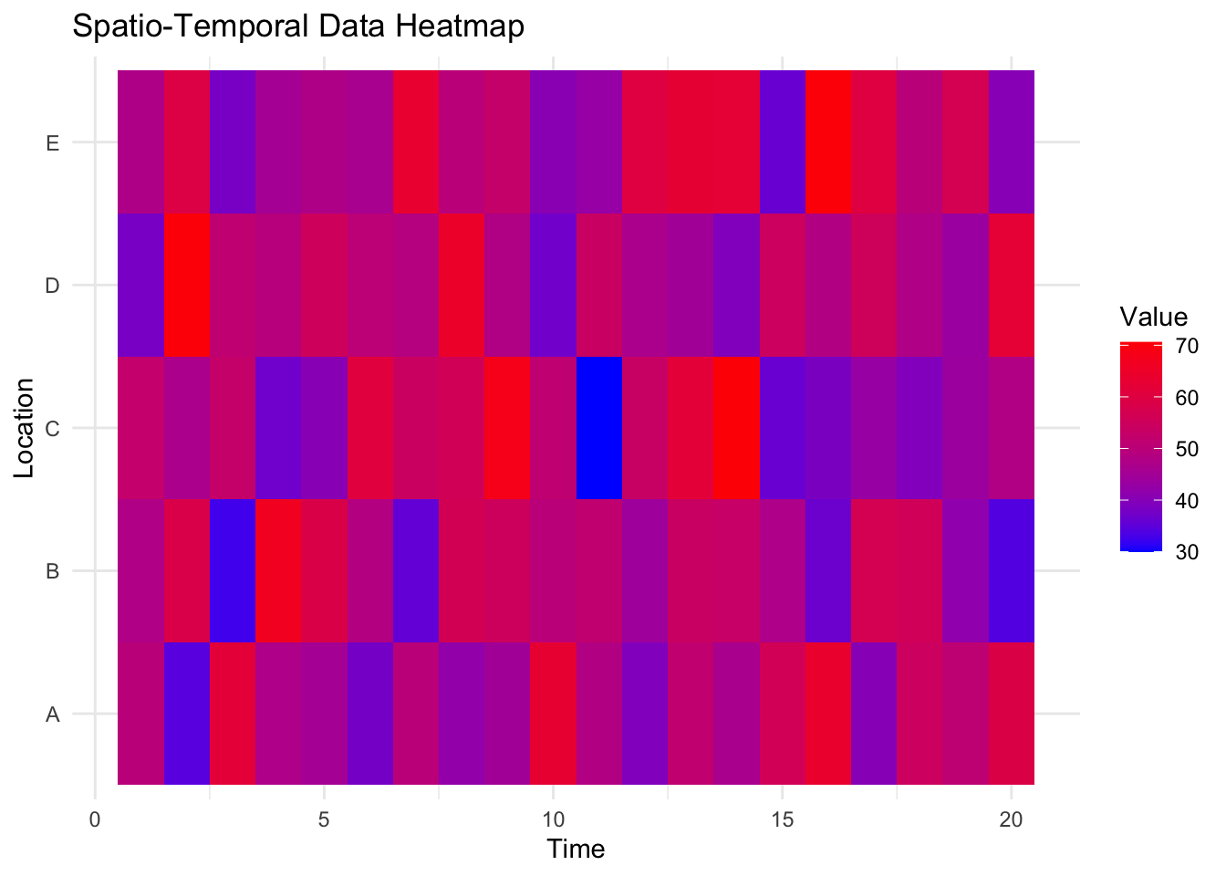
Example

Spatio-temporal data combines time series with geographic variation. The heatmap below illustrates variations in time series values across different locations.

17.6.3 Dynamic panel models

Dynamic panel models blend panel data with lagged dependencies, recognising that each entity’s current outcome depends on its own past values and possibly the past values of other entities. These models might include autoregressive terms across different cross-sectional units, as well as exogenous or endogenous regressors.

Techniques like the Arellano-Bond or Arellano-Bover estimators tackle some of the estimation challenges in dynamic panel settings, especially those arising from correlation between lagged outcomes and unobserved entity-specific effects. While more complex, they offer powerful insights by accommodating both cross-entity differences and time-lagged effects.

Dynamic panel models incorporate ideas from ARIMA, where the past states influence the present, while managing the extra layer of cross-sectional variation. Like any sophisticated approach, success in using these methods depends on thorough exploration of assumptions, possible stationarity issues, and diagnostic testing.

17.6.4 Forecasting across panels with varying dynamics

In some cases, each entity in a panel dataset follows its own unique time series pattern, whether that be ARIMA, SARIMA, or another forecasting method. Varying dynamics means that while these processes differ between entities, they still share some common features. To account for this, we can use hierarchical or pooled forecasting methods, which allow models to share some information while still capturing differences between entities.

One approach is multi-level or hierarchical time series forecasting, where parameters are estimated at two levels:

• A pooled level, which captures overall trends across all entities.
• An entity-specific level, which accounts for unique variations in each case.

This method balances flexibility with shared insights, ensuring that each forecast reflects both individual characteristics and wider patterns across the dataset.

Although these techniques can be complex, they are particularly valuable in areas like marketing and retail forecasting, where multiple products may have their own seasonal trends and sales patterns but are also influenced by broader market conditions. By modelling these layered relationships, we can create forecasts that reflect both ‘big-picture’ trends and fine details.