Introduction
Structural Equation Modelling (SEM) combines factor analysis and multiple regression to analyse complex relationships between variables. SEM allows us to test theoretical models by examining both direct and indirect relationships between observed (measured) variables and unobserved (latent) constructs.
Why is SEM useful?
It’s particularly valuable when multiple interrelated variables need to be analysed simultaneously. It enables us to:
Test complex theoretical frameworks;
Account for measurement error in analyses;
Examine both direct and indirect effects; and
Compare alternative models using goodness-of-fit indices.
While more complex than some traditional methods, SEM provides a robust framework for testing hypotheses about relationships between variables and for evaluating theoretical models against empirical data.
Path analysis and SEM
You may have heard the term “path analysis” before, and wondered about the relationship between path analysis and SEM.
“Path analysis” is a precursor to, and fundamental component of SEM.
While path analysis works with observed variables only, SEM extends this by incorporating latent variables (theoretical constructs) and measurement models. This evolution marked a significant advancement in statistical modelling, allowing the testing of more complex theoretical relationships.
Visualisation of a Path Analysis - note that it only includes observed variables, not latent variables
“Observed” variables are things we can directly measure in some way. “Latent” variables are theoretical constructs we cannot directly measure but infer from multiple observed variables.
Examples include:
Depression – not measured directly, but assessed through multiple symptoms and behavioural markers
Intelligence – not measured directly, but assessed through various test scores
Job satisfaction – not measured directly, but inferred from multiple questions about workplace experiences
Latent and Observed Variables
Introduction
Structural Equation Modelling (SEM) allows us to analyse relationships between different types of variables.
In SEM, there are two categories of variable:
Latent variables: Theoretical constructs that cannot be directly measured but are inferred from multiple observed variables.
Observed variables: Measurable indicators that represent directly collected data. They may act as proxies for latent variables or appear as standalone variables in the model.
Notice how this idea is similar to factor analysis, which also assumes there are latent factors underpinning observed responses.
In SEM diagrams, latent variables are often depicted as circles, while observed variables are represented as rectangles. Arrows indicate relationships: one-headed arrows typically show causal paths, and two-headed arrows indicate correlations.
Latent Variables and SEM
Introduction
Latent variables, often called “unobserved” or “hidden” variables, are a defining feature of SEM. They represent abstract concepts (e.g., intelligence, anxiety, market sentiment) inferred from observed data.
Role of latent variables in SEM
Latent variables form a conceptual bridge between theory and data. They help account for measurement error by allowing a distinction between the underlying construct and the imperfect indicators that measure it. This makes SEM particularly useful in fields where the phenomena of interest are inherently unobservable (e.g., psychological traits, sociological constructs).
Conceptual foundations
The assumption underlying latent variables is that multiple observed indicators reflect a shared underlying construct. For example, if we hypothesize a latent variable “job satisfaction,” we might measure it using several survey items (e.g., pay satisfaction, work environment, teamwork). Each indicator captures a facet of the broader theoretical concept.
Estimation and Identification
Latent variables and their relationships to observed indicators are expressed through equations in SEM. Parameters (factor loadings, structural coefficients) are often estimated using maximum likelihood (ML) or Bayesian methods. A key challenge is model identification. A model is identified if there is enough information in the data to estimate unique parameter values. Common rules of thumb include having at least three good indicators for each latent variable.
Role in structural relationships
In SEM, latent variables can act as predictors and outcomes, forming complex networks of causal relationships. For instance, “academic motivation” could predict “academic performance,” which then predicts “career satisfaction.” SEM can also model indirect effects, such as “parental support” influencing “academic performance” through “self-efficacy.”
Some practical considerations
Because latent variables are not directly measurable, strong theoretical justification and carefully chosen indicators are essential. Validity and reliability must be assessed (e.g., through model fit indices, reliability measures) to ensure that the latent variables accurately capture the constructs.
Measurement models
In SEM, measurement models specify how latent variables are linked to observed indicators. This is often done via confirmatory factor analysis (CFA). Good measurement models ensure that each observed indicator provides useful information about the underlying latent construct.
Observed Variables
Introduction
Observed variables (or “manifest” variables) are directly measured data points—such as test scores, questionnaire items, or physiological readings. They anchor theoretical constructs to empirical reality.
Observed variables in SEM
Observed variables play three main roles in SEM:
Indicators of latent variables
- E.g., questionnaire items about mood or energy levels could indicate “depression.”
Exogenous variables (independent variables)
- E.g., parental income or hours spent studying might predict latent constructs or other observed measures.
Endogenous variables (dependent variables)
- E.g., test scores influenced by latent or observed predictors.
Theoretical implications of observed variables
Choosing the right observed variables is crucial. They must align with the constructs and hypotheses under investigation. For instance, if the theoretical model suggests that “emotional intelligence” predicts “job performance,” the observed indicators chosen (e.g., questionnaire items for EI, supervisor ratings for performance) must be valid and reliable representations of those constructs.
Indicator reliability
Indicator reliability refers to how consistently an observed variable measures what it is intended to measure. In SEM, reliability can be evaluated in several ways:
Cronbach’s alpha or composite reliability for sets of indicators
Factor loadings in the measurement model (indicators should load strongly on the latent factor)
Residual variances to see how much unexplained variation remains
High reliability is critical: if indicators do not consistently reflect the underlying construct, estimates of relationships between variables can be biased or unstable.
Model Specification in SEM
Introduction
Model specification in SEM involves translating a theoretical framework into a structured set of relationships among variables. Good specification accurately reflects the hypotheses and ensures testable predictions.
What is model specification?
Model specification is the process of defining:
Variables
- Latent variables (unobservable) and observed variables (directly measurable).
Relationships
- One-headed arrows to imply causation, two-headed arrows to imply correlation.
Constraints
- Which parameters are free to be estimated (e.g., path coefficients) and which are fixed.
Measurement models and structural models
Measurement Model
Structural Model
Describes how latent (or sometimes observed) variables relate to each other.
E.g., “Team Cohesion” → “Match Performance.”
Steps in model specification
Develop a Theoretical Framework
- Base your model on existing theory or research.
Create a Path Diagram
- Use circles for latent variables and rectangles for observed variables.
Write the Equations
- Each path corresponds to an equation (e.g.,
Performance = β1*(Cohesion) + ε).
Specify Parameters
- Decide which paths are estimated and which are fixed at 0 or at a specific value.
Check Identifiability
- Ensure there are enough constraints and data to estimate the model’s parameters uniquely.
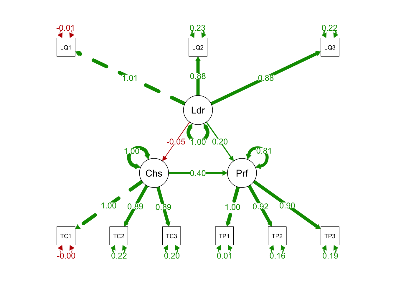
Example: Model specification in rugby
Imagine you’re studying factors that influence Team Performance in rugby. You hypothesise:
Observed variables could include:
Survey items for Team Cohesion (e.g., “Trust among players,” “Shared goals”).
Coach ratings and player feedback for Leadership Quality.
Match outcomes or points scored for Team Performance.
Model specification means defining these latent variables, linking them to observed indicators, and laying out the causal paths.
This is lavaan 0.6-20
lavaan is FREE software! Please report any bugs.
Warning: lavaan->lav_object_post_check():
   some estimated ov variances are negative
lavaan 0.6-20 ended normally after 40 iterations

  Estimator                                         ML
  Optimization method                           NLMINB
  Number of model parameters                        21

  Number of observations                           200

Model Test User Model:

  Test statistic                                34.271
  Degrees of freedom                                24
  P-value (Chi-square)                           0.080

Model Test Baseline Model:

  Test statistic                              2013.860
  Degrees of freedom                                36
  P-value                                        0.000

User Model versus Baseline Model:

  Comparative Fit Index (CFI)                    0.995
  Tucker-Lewis Index (TLI)                       0.992

Loglikelihood and Information Criteria:

  Loglikelihood user model (H0)              -1704.437
  Loglikelihood unrestricted model (H1)      -1687.301

  Akaike (AIC)                                3450.874
  Bayesian (BIC)                              3520.139
  Sample-size adjusted Bayesian (SABIC)       3453.608

Root Mean Square Error of Approximation:

  RMSEA                                          0.046
  90 Percent confidence interval - lower         0.000
  90 Percent confidence interval - upper         0.079
  P-value H_0: RMSEA <= 0.050                    0.537
  P-value H_0: RMSEA >= 0.080                    0.044

Standardized Root Mean Square Residual:

  SRMR                                           0.039

Parameter Estimates:

  Standard errors                             Standard
  Information                                 Expected
  Information saturated (h1) model          Structured

Latent Variables:
                   Estimate  Std.Err  z-value  P(>|z|)   Std.lv  Std.all
  Leadership =~
    LQ1               1.000                               0.946    1.005
    LQ2               0.975    0.042   23.272    0.000    0.922    0.877
    LQ3               0.974    0.041   23.853    0.000    0.922    0.883
  Cohesion =~
    TC1               1.000                               1.024    1.002
    TC2               0.966    0.039   24.543    0.000    0.989    0.886
    TC3               1.003    0.039   25.570    0.000    1.027    0.895
  Perf =~
    TP1               1.000                               1.073    0.997
    TP2               0.986    0.034   29.086    0.000    1.059    0.917
    TP3               1.005    0.038   26.665    0.000    1.078    0.900

Regressions:
                   Estimate  Std.Err  z-value  P(>|z|)   Std.lv  Std.all
  Cohesion ~
    Leadership       -0.052    0.076   -0.688    0.491   -0.048   -0.048
  Perf ~
    Leadership        0.223    0.072    3.098    0.002    0.197    0.197
    Cohesion          0.424    0.067    6.326    0.000    0.405    0.405

Variances:
                   Estimate  Std.Err  z-value  P(>|z|)   Std.lv  Std.all
   .LQ1              -0.009    0.018   -0.528    0.597   -0.009   -0.010
   .LQ2               0.255    0.030    8.383    0.000    0.255    0.231
   .LQ3               0.240    0.029    8.228    0.000    0.240    0.220
   .TC1              -0.004    0.018   -0.237    0.813   -0.004   -0.004
   .TC2               0.269    0.032    8.472    0.000    0.269    0.216
   .TC3               0.263    0.032    8.220    0.000    0.263    0.200
   .TP1               0.006    0.017    0.345    0.730    0.006    0.005
   .TP2               0.213    0.027    7.925    0.000    0.213    0.159
   .TP3               0.273    0.032    8.489    0.000    0.273    0.190
    Leadership        0.894    0.090    9.913    0.000    1.000    1.000
   .Cohesion          1.046    0.106    9.893    0.000    0.998    0.998
   .Perf              0.928    0.095    9.793    0.000    0.805    0.805
Parameter Estimation in SEM
Introduction
After specifying a model, the next step is to estimate its parameters (e.g., factor loadings, path coefficients). These estimates tell us how strongly variables are related and help us evaluate whether our theoretical model aligns with the data.
Model parameters
Model parameters in SEM typically include:
Factor loadings: how strongly each observed indicator relates to its latent variable.
Regression weights (path coefficients): the strength of direct effects between variables.
Covariances or correlations: the relationships between exogenous variables or error terms.
Variances: how much each variable varies, including error or residual variance.
Estimation techniques
Common estimation methods include:
Maximum Likelihood (ML): The most widely used. Assumes multivariate normality and aims to find parameter values that maximise the likelihood of observing the data.
Weighted Least Squares (WLS): Often used for categorical or non-normal data. Minimises weighted squared differences between observed and model-implied correlations.
Bayesian Estimation: Incorporates prior distributions for parameters, updates these with observed data, and produces posterior distributions.
The choice of estimator depends on the data structure (e.g., continuous vs. ordinal, normal vs. non-normal) and the research question.
Goodness-of-fit
Goodness-of-fit tells us how well the estimated model reproduces the observed data. While specific fit indices appear in the next section, an overall principle is to ensure that the model’s predicted relationships closely match the actual relationships in the dataset. Poor fit often indicates that key paths or constructs are missing, or that the theoretical model is not supported by the data.
Model Fit and Evaluation
Introduction
Once parameters are estimated, we need to assess how well the model fits the data. Fit indices help determine whether the theoretical model is plausible or needs revision.
Global fit indices
Common global fit indices include:
Chi-square test (χ²): Tests the null hypothesis that the model’s implied covariance matrix equals the observed covariance matrix. Sensitive to sample size.
Root Mean Square Error of Approximation (RMSEA): Assesses how well the model would fit the population’s covariance matrix. Values ≤ .06 are often considered good.
Comparative Fit Index (CFI) and Tucker-Lewis Index (TLI): Compare the specified model to a baseline (null) model. Values close to 1 indicate better fit.
Standardized Root Mean Square Residual (SRMR): The average discrepancy between observed and predicted correlations.
Assessment of ‘local fit’
Local fit involves scrutinising individual parameters and residuals:
Residuals: Differences between observed and predicted correlations or covariances. Large residuals suggest misfit in specific parts of the model.
Modification indices: Indicate how much model fit would improve by freeing a constrained (fixed) parameter. Can guide model refinement, though it’s best to have theoretical justification for any changes.
Model parsimony
Parsimony implies using the simplest model that adequately explains the data. Overly complex models may fit well but risk overfitting, while overly simple models might miss important pathways. Common measures, like the Akaike Information Criterion (AIC), balance fit and complexity.
Model Validation and Generalisation
Introduction
Even if a model fits well in one dataset, we want to ensure it generalises to other samples and contexts. Validation procedures help confirm the robustness of the findings.
Cross-Validation
Cross-validation involves testing the model on a separate dataset or on different subsets of the same dataset (e.g., split-half validation). If the model fits similarly in new data, it has stronger support for generalisability.
Measurement Invariance
Measurement invariance assesses whether the same latent variables are measured equivalently across groups (e.g., by gender or culture). If invariance holds, group comparisons of latent variable means and relationships are more valid.
Replication
Replication involves re-running the same model with new data or in a different context. Repeated successful replications increase confidence that the findings are not sample-specific and truly reflect underlying relationships.