9 Discriminant Analysis
9.1 Introduction
Discriminant Analysis is used in machine learning and data analysis for both classification and dimensionality reduction.
It was first developed by Ronald Fisher in 1936, and has become an important tool in multivariate statistics.
It helps identify the combination of features that best separates different classes of objects or events, making it particularly valuable in pattern recognition and predictive modelling.
Think of discriminant analysis like a smart sorting system. Imagine you have a basket of fruits (apples, oranges, and bananas) and you want to create a rule to automatically sort them. You might use features like colour, shape, and size to tell them apart.
Discriminant analysis does exactly this - it creates a mathematical rule that looks at different characteristics to separate items into their correct groups.
The primary goal of discriminant analysis is to establish a mathematical rule or function that can classify observations into pre-defined groups based on their characteristics.
9.2 Classification
Discriminant analysis is primarily used for classification tasks, where the goal is to assign observations to predefined classes based on their predictor variables.
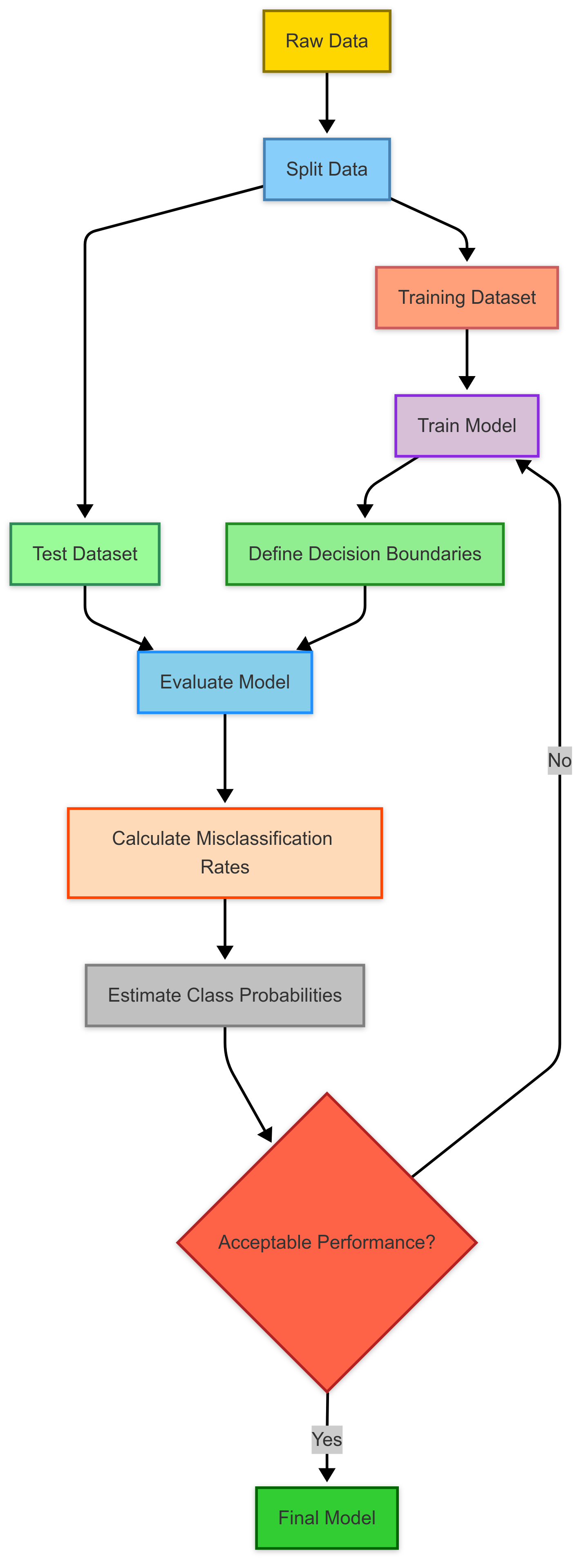
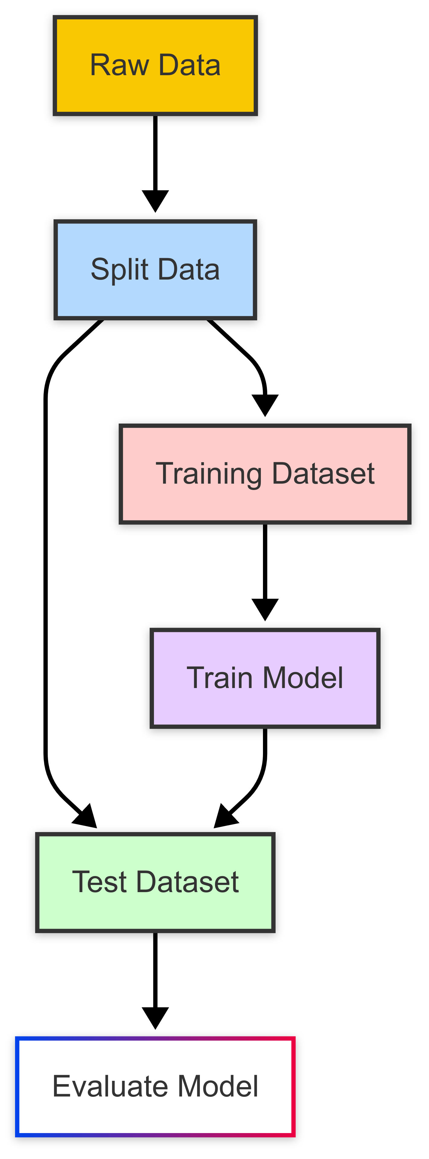
This involves splitting the dataset into training and test sets, defining decision boundaries, calculating misclassification rates, and estimating the probabilities of class membership.
The effectiveness of the model hinges on its ability to classify observations accurately.
This flowchart illustrates the typical classification process, from data preparation through model evaluation and refinement.
Training dataset
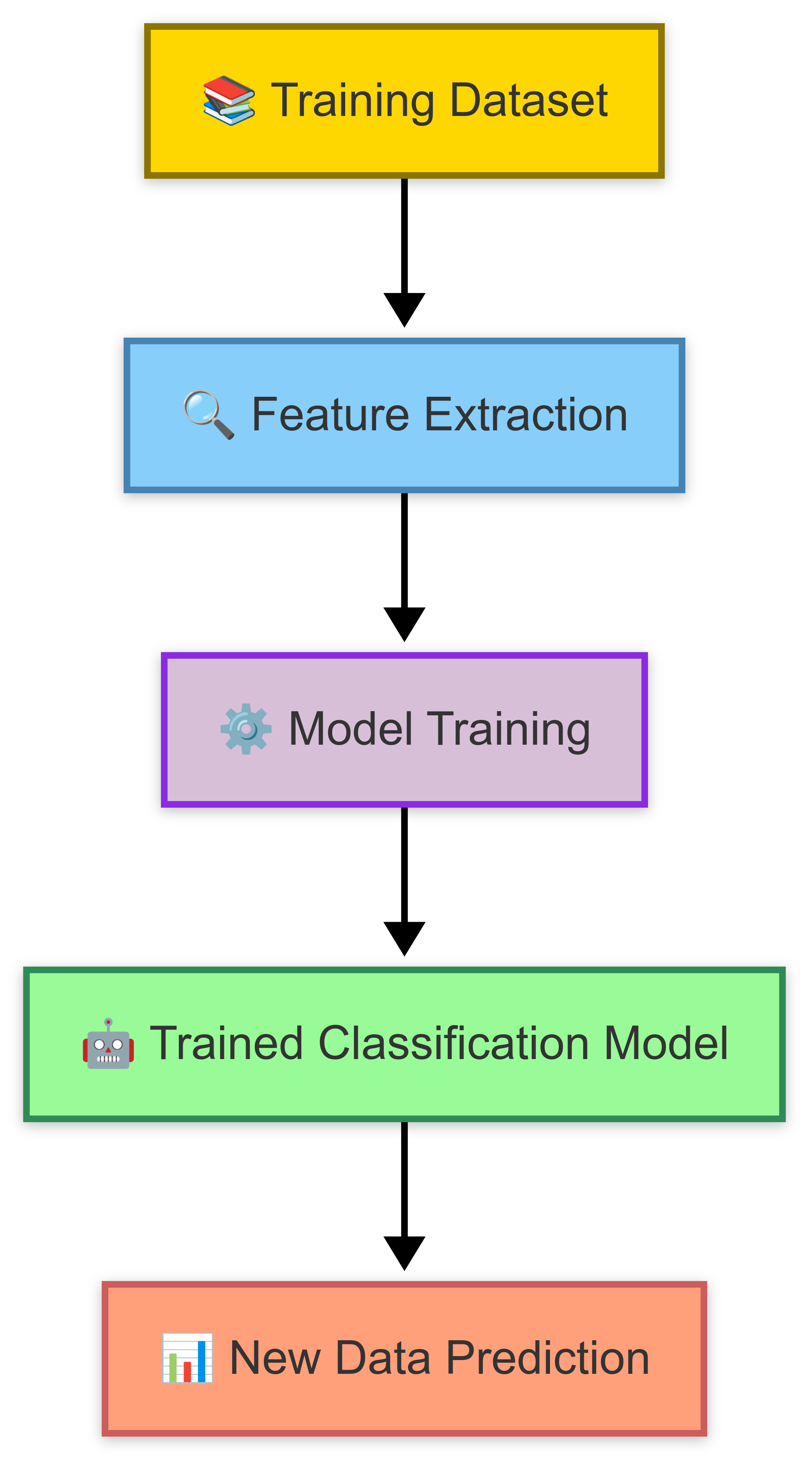
The ‘training dataset’ is where the model learns the patterns and relationships between predictor variables and class memberships.
A training dataset is a collection of labeled data used to train classification models.
By ‘labelled’, we mean that it has a known outcome (e.g., ‘apple’, ‘orange’).
Usually, we’d divide our dataset into two parts; training and testing. We do this before undertaking any analysis.
The training set provides the foundation for the model to learn patterns and relationships between input features (independent variables) and their corresponding outputs (dependent variables or classes).
Each data point in the training dataset consists of feature values and a known label, which the model uses to iteratively adjust its parameters through algorithms like gradient descent, aiming to minimise the error in its predictions.
Once we’ve trained our classification model, we can then ‘test’ the effectiveness of our model on a test dataset.
Test dataset
The test dataset is used to evaluate the model’s performance on new, unseen data. It contains observations with known class labels that were not used during training.
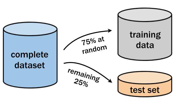
A test dataset is a separate subset of data (usually 25-30% of the complete dataset) which we use to evaluate the performance of a trained machine learning model.
Unlike the training dataset, the test dataset is not used during the learning process. Like the training dataset, it contains labeled data with known outcomes but these were not used during model training.
This enables a direct comparison between the model’s predictions and the actual labels (using metrics such as accuracy, precision, recall, or F1-score). We’ll explore these metrics later in this topic.
Decision boundaries
In Discriminant Analysis, a decision boundary is like an invisible line (or surface, in more dimensions) that separates different classes in a dataset.
When you train a model, it learns the best way to divide the space so that new data points can be correctly classified.
Imagine plotting exam scores for two groups of students; those who pass and those who fail. The decision boundary would be the point where the model decides whether a new student belongs in the “pass” or “fail” category based on their score.
In Linear Discriminant Analysis (LDA), the decision boundary is always a straight line (or plane in higher dimensions). This works well when the data from different classes forms clear, separate clusters.
However, in Quadratic Discriminant Analysis (QDA), the decision boundary can curve, making it more flexible when class distributions are more complex. If two classes overlap in a messy way, a straight-line boundary might not be enough, and QDA’s curved boundaries can do a better job of dividing them.
The key idea is that when new data comes in, the model checks which side of the boundary it falls on and assigns it to the closest class. A well-defined boundary means the model is confident in its decisions, while a poor boundary can lead to misclassifications.
This is why choosing the right type of discriminant analysis depends on how your data is spread out. Sometimes a simple straight line works (LDA), and other times, a more flexible approach is needed (QDA).
Technical explanation
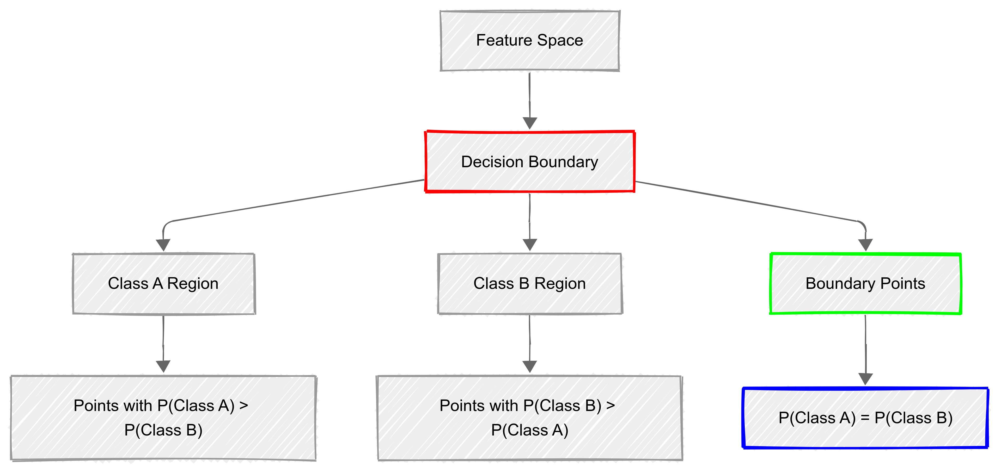
Decision boundaries are determined by the discriminant functions and represent where the probability of belonging to one class equals the probability of belonging to another class.
Key aspects of decision boundaries include:
- They partition the feature space into regions corresponding to different classes;
- The shape depends on the type of discriminant function (linear or quadratic);
- Points lying on the boundary have equal probability of belonging to adjacent classes; and
- The optimal boundary minimises misclassification error in the training data.
Misclassification rates
When we develop classification models, misclassification rates are important tools we can use to assess how often a model makes incorrect predictions.
A lower misclassification rate indicates a more accurate model, while a higher rate suggests room for improvement!
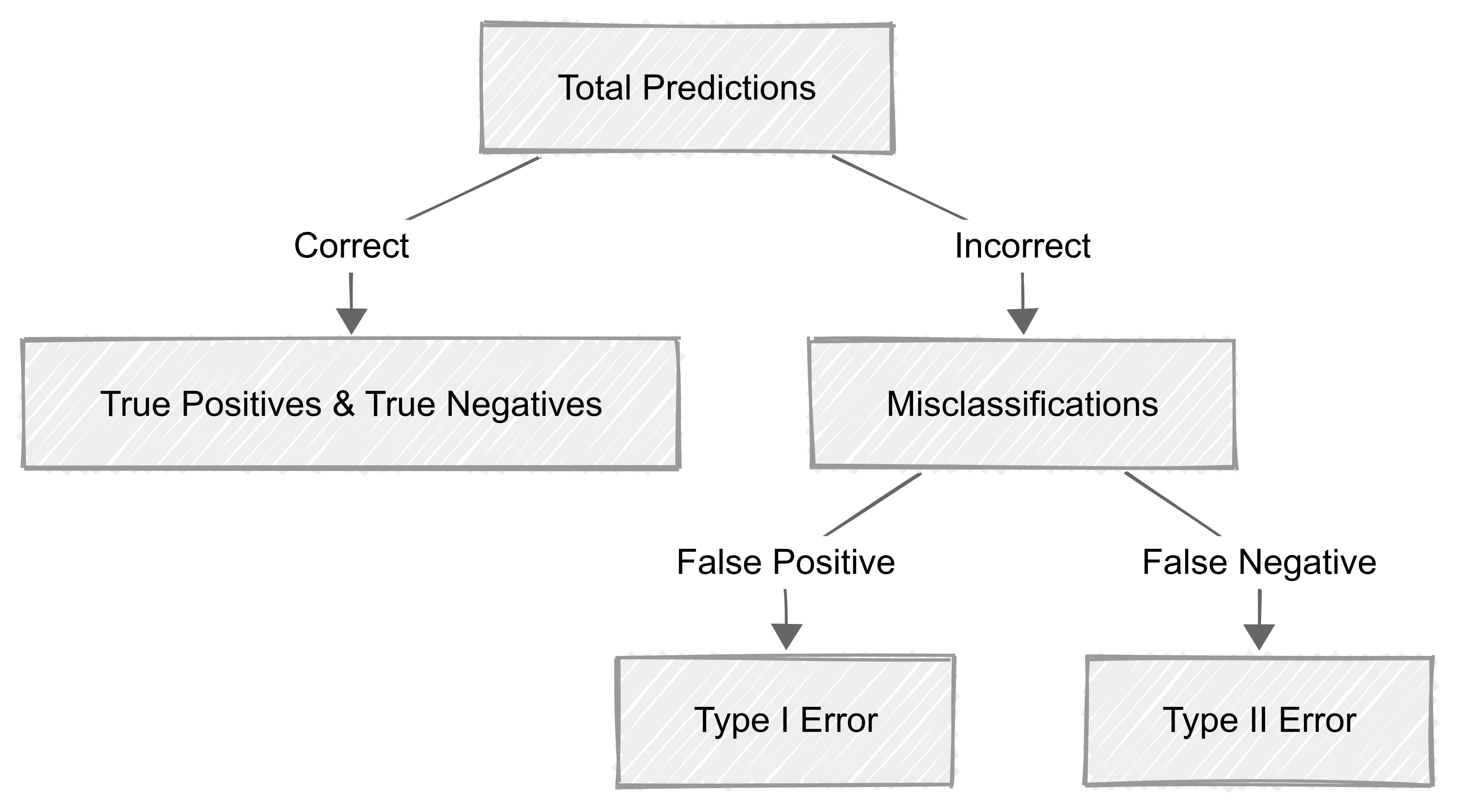
Misclassifications occur when the model incorrectly predicts the class of an observation. These errors are categorised into two main types:
- False Positives (Type I Error): The model incorrectly predicts a positive outcome for a negative case.
- False Negatives (Type II Error): The model incorrectly predicts a negative outcome for a positive case.
Understanding these errors is essential for refining classification models and improving their predictive performance.
Calculating the misclassification rate
The misclassification rate is calculated using the following formula:
\[ \text{Misclassification Rate} = \frac{\text{False Positives} + \text{False Negatives}}{\text{Total Number of Predictions}} \]
It helps us quantify the proportion of incorrect predictions made by a model relative to the total number of predictions.
Visualising misclassification
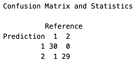
The confusion matrix helps us visualise how ‘well’ our model has performed when applied to the test data:
Reducing misclassification rates
To enhance the accuracy of classification models and minimise misclassification rates, there are a few things we can do:
Feature Engineering and Selection – Choosing the most relevant features improves the model’s ability to distinguish between classes.
Model Tuning and Optimisation – Adjusting hyperparameters can refine the decision boundaries and improve predictions.
Using Ensemble Methods – Techniques like bagging, boosting, and stacking combine multiple models to reduce individual model weaknesses.
Collecting More Training Data – A larger dataset can improve model generalisation and reduce overfitting.
Addressing Class Imbalance – If one class is significantly underrepresented, techniques like oversampling, under-sampling, or synthetic data generation (e.g., SMOTE) can improve performance.
By applying these techniques, we can build more reliable classification models and reduce misclassification rates.
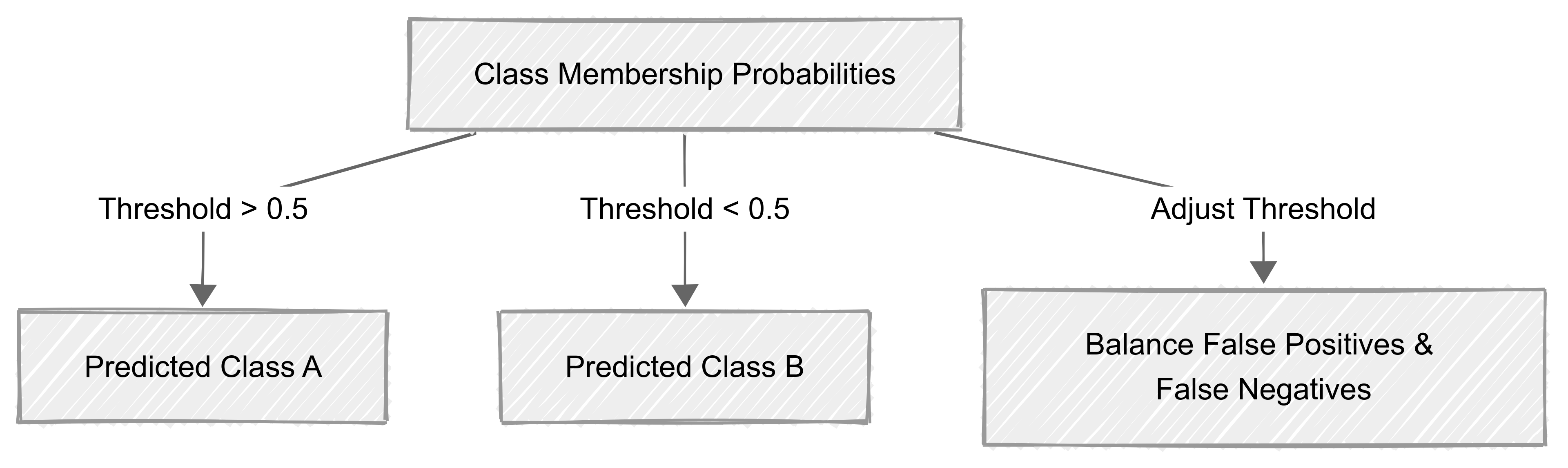
Class membership probabilities
In many classification models, predictions are not just binary labels (e.g., “yes” or “no”) but are accompanied by class membership probabilities.
These probabilities represent the model’s confidence in assigning an observation to a particular class.
For a given observation, a classifier might output:
- 0.85 for Class A
- 0.15 for Class B
This means the model believes the observation belongs to Class A with an 85% confidence level. It belongs to Class B with 15% confidence level.
Class membership probabilities and misclassification
Misclassification often occurs when the model misinterprets class probabilities.
For example, if a model assigns a probability of 0.51 to Class A and 0.49 to Class B, it will classify the observation as Class A, despite a near-even probability distribution.
This can lead to errors, especially in cases where the decision threshold is not well-calibrated.
Adjusting decision thresholds to reduce misclassification
By default, many models classify an observation into the class with the highest probability (typically using a 0.5 threshold).
However, adjusting the threshold can help reduce misclassification rates, particularly when false positives or false negatives have different consequences.
For example:
In medical diagnostics, a lower threshold (e.g., 0.3) for detecting a serious disease might reduce false negatives, ensuring more at-risk patients receive further testing.
In fraud detection, a higher threshold (e.g., 0.7) might reduce false positives, preventing unnecessary account restrictions.
Visualising class probabilities
A ROC curve (Receiver Operating Characteristic curve) is often used to visualise the trade-off between sensitivity (true positive rate) and specificity (true negative rate) at different probability thresholds.
9.3 Discriminant Functions
The discriminant function is a mathematical representation that distinguishes between classes.
In simple terms, a discriminant function is like a mathematical sorting tool that helps us put things into different groups based on their characteristics.
Just like we might sort foods into “sweet” and “sour” based on their taste, a discriminant function uses measurements or features to automatically classify items into distinct categories.
For example, it could help separate emails into “spam” and “not spam” based on certain words they contain, or classify flowers into different species based on their petal length and width.
The discriminant function can be linear or quadratic, depending on the data and assumptions. The function assigns weights to features in order to maximise separation between classes.
Eigenvalues and class separation metrics help us to evaluate the discriminative ‘power’ of the function.
Linear Discriminant Function (LDF)
The Linear Discriminant Function (LDF) is widely used in machine learning, statistics, and pattern recognition for classification tasks.
How does LDF work?
The LDF finds a linear boundary that best separates two or more classes based on their features. It does this by:
- Computing the mean vectors for each class.
- Finding a projection line that maximises the separation between the means of the classes while minimising the variance within each class.
- Drawing a decision boundary, which is typically a straight line (in 2D) or a hyperplane (in higher dimensions).
For a binary classification problem, the LDF is expressed as:
\[ g(x) = w_0 + w_1x_1 + w_2x_2 + ... + w_nx_n \]
If \(g(x) > 0\), classify as Class 1.
If \(g(x)≤0\), classify as Class 2.
Visual example
This figure shows how Linear Discriminant Analysis (LDA) separates two classes using a straight-line decision boundary (dashed line).
The model finds the best way to divide the space so that most points from each class fall on the correct side.
Some points may still be misclassified, especially if the classes overlap, but the boundary represents the best possible linear separation based on the data.
-01.png)
Practical Example: Email Spam Detection
Imagine you’re building a classifier to detect spam emails.
You extract two key features that you think are important:
\(x_1\) = Frequency of the word “free” in the email
\(x_2\) = Number of capitalised words in the email
Using a training dataset, the classifier learns weights (\(w_1, w_2)\) and a bias term (\(w_0\)) to create a linear decision boundary that distinguishes spam from non-spam emails.
\[ g(x) = w_0 + w_1x_1 + w_2x_2 \]
So for any given email:
- If \(g(x) > 0\) classify it as Spam.
- If \(g(x)≤0\), classify it as Not Spam.
9.4 Example Decision Rule
Let’s say the classifier has learned the following equation
\[ g(x) = -5 + 2x_1 + 3x_2 \]
If an email has \(x_1 = 3\) occurrences of “free” and \(x_2 = 1\) capitalised word:
\[ g(3,1) = -5 + (2*3) + (3*1) = -5 + 6 + 3 = 4 \]
Since \(g(x)\>0\) the email is classified as Spam.
Advantages of LDF
✅ Efficient on Linearly Separable Data: It works well when classes can be separated by a straight line or hyperplane.
✅ Interpretable: Unlike deep learning models, LDF provides a clear mathematical decision boundary.
✅ Fast Computation: Makes it suitable for real-time applications like fraud detection or medical diagnosis.
✅ Dimensionality Reduction: Used in Linear Discriminant Analysis (LDA) to project high-dimensional data onto a lower-dimensional space while preserving class information.
Limitations of LDF
🚫 Doesn’t Handle Non-Linearly Separable Data Well: If the classes are intertwined, LDF struggles to find a good boundary.
🚫 Sensitive to Outliers: A few extreme data points can skew the decision boundary.
🚫 Assumes Gaussian Distributions: Works best when data is normally distributed within each class.
Solution for Non-Linearly Separable Data
If our data is not linearly separable, we can:
Use Kernel Methods: Transform data into a higher-dimensional space (as done in Support Vector Machines).
Apply Non-Linear Models: Neural networks or decision trees handle complex patterns better.
Quadrant Discriminant Function
The Quadratic Discriminant Function (QDF) is an extension of the Linear Discriminant Function (LDF) that allows for non-linear decision boundaries between classes.
Unlike LDF, which assumes equal covariance structures across classes, QDF does not assume equal covariance and models each class separately.
The decision rule is based on a quadratic function of the form:
\[ g(x) = x^T W x + v^T x + w\]
where:
- \(x\) is the feature vector,
- \(W\) is a quadratic term,
- \(v\) is a linear term,
- \(w\) is a constant term.
Because of the quadratic term (\(x^T W x\)), QDF can capture curved, elliptical, or more complex decision boundaries.
.png)
Visual example
This graph shows how Quadratic Discriminant Analysis (QDA) separates two classes using a curved decision boundary (dashed line).
Unlike LDA, which assumes a straight-line separation, QDA adapts to more complex class distributions, making it more effective when the data is not evenly spread.
QDF over LDF?
✅ Handles Non-Linearly Separable Data- Unlike LDF, which assumes a straight-line boundary, QDF creates curved boundaries.
✅ Accounts for Different Class Covariances – Each class can have a unique variance structure, improving accuracy.
✅ Better for Complex Datasets – Useful when class distributions are not well-separated by a linear boundary.
🚫 More Computationally Expensive** – QDF requires estimating separate covariance matrices for each class.
🚫 More Prone to Overfitting – Especially when sample sizes are small.
Practical Example: Image Classification of Digits
Imagine we want to classify handwritten digits based on two extracted features:
\(x_1\) = Intensity of ink in the top-left region
\(x_2\) = Symmetry of the digit
A QDF model can be trained on a labeled dataset where the covariance structure varies across different digit classes. Because handwritten digits exhibit curved decision boundaries, QDF is more effective than LDF in this case.
10 Visualising QDF Decision Boundaries
This is a decision boundary plot using Quadratic Discriminant Analysis (QDA) to classify three classes. It highlights the difference between linear and quadratic decision regions.
.png)
Key Takeaways
Non-Linear Boundaries: Unlike LDF, which creates straight-line separations, QDF generates curved decision boundaries. This allows it to handle more complex class distributions.
More Flexibility: Each class is assigned its own covariance structure, making it better suited for problems where data is not evenly distributed.
Comparison with LDF: If the classes were truly linearly separable, LDF would work just as well, but in cases like this where distributions overlap and curve, QDF performs better.
When to Use LDF vs. QDF?
| Criteria | Linear Discriminant Function (LDF) | Quadratic Discriminant Function (QDF) | ||||
| Decision Boundary | Linear (Straight Line) | Quadratic (Curved) | ||||
| Assumption on Covariance | Assumes equal covariance for all classes | Allows different covariance per class | ||||
| Computational Efficiency | Faster, fewer parameters | More complex, needs larger datasets | ||||
| Performance on Small Datasets | More stable, less prone to overfitting | Prone to overfitting if data is sparse | ||||
Feature coefficients
When using discriminant functions (such as Linear Discriminant Analysis (LDA) and Quadratic Discriminant Analysis (QDA)), we often want to understand how each feature (variable) contributes to classification.
This is done through feature coefficients, which determine how strongly each feature influences the decision boundary between classes.
- Large coefficients mean a feature is important for classification.
- Positive coefficients increase the likelihood of a particular class.
- Negative coefficients decrease the likelihood of a particular class.
- Near-zero coefficients mean the feature has little effect.
By analysing these coefficients, we can interpret the model and understand what drives the classification decision.
11 Understanding class separation
In discriminant analysis, class separation refers to how well a model can distinguish between different categories.
Remember: the goal of a classification model is to maximise separation so that data points from different classes do not overlap significantly.
Well-separated classes → Model performs well with high accuracy.
Overlapping classes → Model struggles, leading to misclassifications.
Different discriminant functions handle class separation in different ways:
Linear Discriminant Analysis (LDA): Assumes that classes can be separated by a straight line (or hyperplane in higher dimensions).
Quadratic Discriminant Analysis (QDA): Allows for curved decision boundaries, providing better separation when class distributions overlap in a non-linear way.
Measuring class separation
To quantify class separation, we use:
Between-Class Variance vs. Within-Class Variance
Between-class variance: Measures how far apart class means are.
Within-class variance: Measures how spread out each class is.
A good classification model aims for high between-class variance and low within-class variance.
Mahalanobis Distance
Measures distance between class means, considering covariance structure.
Larger distances indicate better separation.
Linear Discriminant Ratio (LDR)
Ratio of between-class variance to within-class variance.
Higher values mean better separation.
12 Visualising class separation
13 Feature Coefficients in LDA
LDA assumes that class separation is linear and assigns a weight (coefficient) to each feature in the decision function:
\[ g(x) = w_0 + w_1x_1 + w_2x_2 + ... + w_nx_n \]
where:
- \(w_0\) is the intercept (bias),
- \(w_1, w_2, ..., w_n\) are the feature coefficients,
- \(x_1, x_2, ..., x_n\) are the feature values.
The higher the absolute value of \(w_i\) the more influence that feature has on classification.
Feature Coefficients in QDA
QDA extends LDA by allowing curved decision boundaries. Instead of a single weight per feature, it also includes quadratic terms to account for different covariance structures.
The discriminant function for QDA is:
\[g(x) = x^T W x + v^T x + w\]
This means each feature has both linear and quadratic coefficients, making the interpretation more complex but allowing for non-linear class separation.
14 Key Takeaways
- Feature coefficients determine how much each variable influences classification.
- LDA uses a linear function, while QDA introduces quadratic terms for more flexibility.
- Visualising feature coefficients helps in understanding feature importance.
.png)
- The density plot shows how well LDA separates the classes.
- Non-overlapping peaks → Classes are well-separated.
- Overlapping peaks → More misclassifications expected.
Key Takeaways
- Class separation determines how easily a model can classify new data.
- LDA provides linear boundaries, while QDA allows non-linear separation.
- Visualising class separation in LDA space helps identify model performance.
In discriminant analysis, eigenvalues indicate how much of the variance in the dependent variables is explained by each discriminant function.
Eigenvalues and eigenvectors are fundamental concepts in linear algebra and are often used in data analysis, especially in PCA (Principal Component Analysis) and its related techniques.
In discriminant analysis, they represent the ratio of between-group variance to within-group variance for each discriminant function.
An eigenvalue greater than 1.0 indicates that the discriminant function accounts for more variance than could be expected by chance. The larger the eigenvalue, the stronger the discriminating power of that function.
Key points
- They help determine which discriminant functions are most important for separating groups
- The sum of eigenvalues equals the total variance in the discriminant scores
- The proportion of an eigenvalue to the sum of all eigenvalues indicates the relative importance of the corresponding discriminant function
The first discriminant function typically has the largest eigenvalue, meaning it accounts for the maximum separation between groups. Each subsequent function explains progressively less of the remaining variance.
15 Mathematical expression
\[λ = \\frac{\\text{Between-group variability}}{\\text{Within-group variability}}\]
where \(λ\) (lambda) represents the eigenvalue for a given discriminant function.
.png)
What these plots show
Class Separation in LDA Space – Shows how LDA projects data onto a new axis for separation.
If eigenvalues are large, the classes are well-separated.
If eigenvalues are small, the classes overlap more.
Eigenvalues of Discriminant Functions – Shows the importance of each discriminant axis.
The first function has the largest eigenvalue, meaning it explains most of the separation.
The second function (if present) explains less variance.
Key takeaways
Larger eigenvalues = better class separation.
The first discriminant function is the most important.
Eigenvalues help us rank discriminant functions by importance.