5 Cluster Analysis

5.1 Introduction

This chapter introduces the technique of cluster analysis, a statistical approach that attempts to group similar objects together while keeping dissimilar objects in different groups.

Cluster analysis is an unsupervised learning method. That is, we do not start with preconceived ideas of how our data might form into clusters. We allow the model to determine this for us.

It help us to identify natural patterns and structures within data, making it valuable for tasks like customer segmentation, image processing, and pattern recognition.

In the figure on the left, the data is un-clustered. The figure on the right indicates how the clustering algorithm has grouped the datapoints based on their similarity and difference to the other datapoints.

The core objective of clustering is to maximise both intra-cluster similarity (objects within the same cluster should be as similar as possible) and inter-cluster differences (objects in different clusters should be as distinct as possible).

5.2 Cluster Analysis - Key Concepts

Imagine a diverse group of individuals engaging in a physical activity intervention. You collect data on their daily steps, their active minutes per day, and their calories burned per day.

By conducting a cluster analysis, you could group the individuals into three clusters or ‘types’, for example:

Cluster One (red - higher calories burned with a range of daily steps),
Cluster Two (green - higher daily steps but moderate calories burned)
Cluster Three (blue - lower daily steps and lower calories burned).

This is really useful, because it helps us start to identify different types of responses on multiple variables, or different groups within our data. This might in turn lead to some further research questions or analysis on those clusters.

Therefore, cluster analysis identifies patterns in our data by organising it into subsets that share common characteristics.

5.2.1 Partitioning vs. Hierarchical models

In cluster analysis, partitioning models and hierarchical models are two different approaches used to group data points based on their similarities.

Difference between hierarchical and partitional clustering.

Partitioning models

Partitioning models divide a dataset into a predefined number of clusters, where each data point belongs to exactly one cluster.

Notice in the figure above that the partitioning model allocates each data point to one of the three clusters.

These models aim to optimise a specific criterion, such as minimising the distance within clusters or maximising the distance between them.

For example, k-means clustering groups data into k clusters by reducing the variation within each cluster;
k-medoids clustering uses actual data points (medoids) as cluster centers, making it less sensitive to outliers.

The result of these methods is a simple, flat structure where all data points are clearly assigned to one of the clusters.

Hierarchical models

In contrast, hierarchical models build a tree-like structure, called a dendrogram, which shows how data points can be grouped together at various levels.

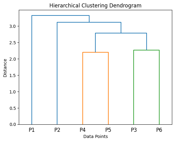
In the figure above, the hierarchical clustering process places all the data points into two groups (P1 and P2-6), then further subdivides the second group into P2 and P4-6, and so on. We end up with four clusters, {P1}, {P2}, {P4, P5}, and {P3, P6}.

These models don’t require the user to specify the number of clusters in advance. Instead, hierarchical clustering can work either from the bottom up (agglomerative), merging smaller clusters into larger ones, or from the top down (divisive), splitting large clusters into smaller ones.

Different linkage methods, such as single linkage (based on the nearest points) or complete linkage (based on the furthest points), determine how distances between clusters are calculated. The dendrogram provides a visual representation of the clusters, and the number of clusters can be decided later by cutting the tree at a particular level.

How are they different?

The key difference between these methods lies in their approach and outcomes.

Partitioning models are more straightforward, assigning each data point to a single cluster and often working well when the number of clusters is already known.

However, they’re somewhat limited in that they typically find spherical clusters, and they can be sensitive to the starting conditions and outliers in our data.

Hierarchical models, on the other hand, are more flexible, allowing for nested groupings and identifying clusters of varying shapes and sizes.

They’re particularly useful for exploratory analysis when the number of clusters isn’t clear, although they are more computationally demanding, especially with large datasets.

How to choose which model

Choosing between partitioning and hierarchical models depends on the specific requirements of your analysis.

Partitioning methods are faster and more efficient for large datasets when you know the number of clusters needed, making them suitable for simpler problems.
Hierarchical models, while computationally heavier, offer greater flexibility and insight into the structure of the data, making them ideal for uncovering complex relationships or nested patterns.

Both approaches have their strengths; understanding their differences helps in selecting the right method for the task at hand.

5.2.2 Density-based vs. distribution-based models

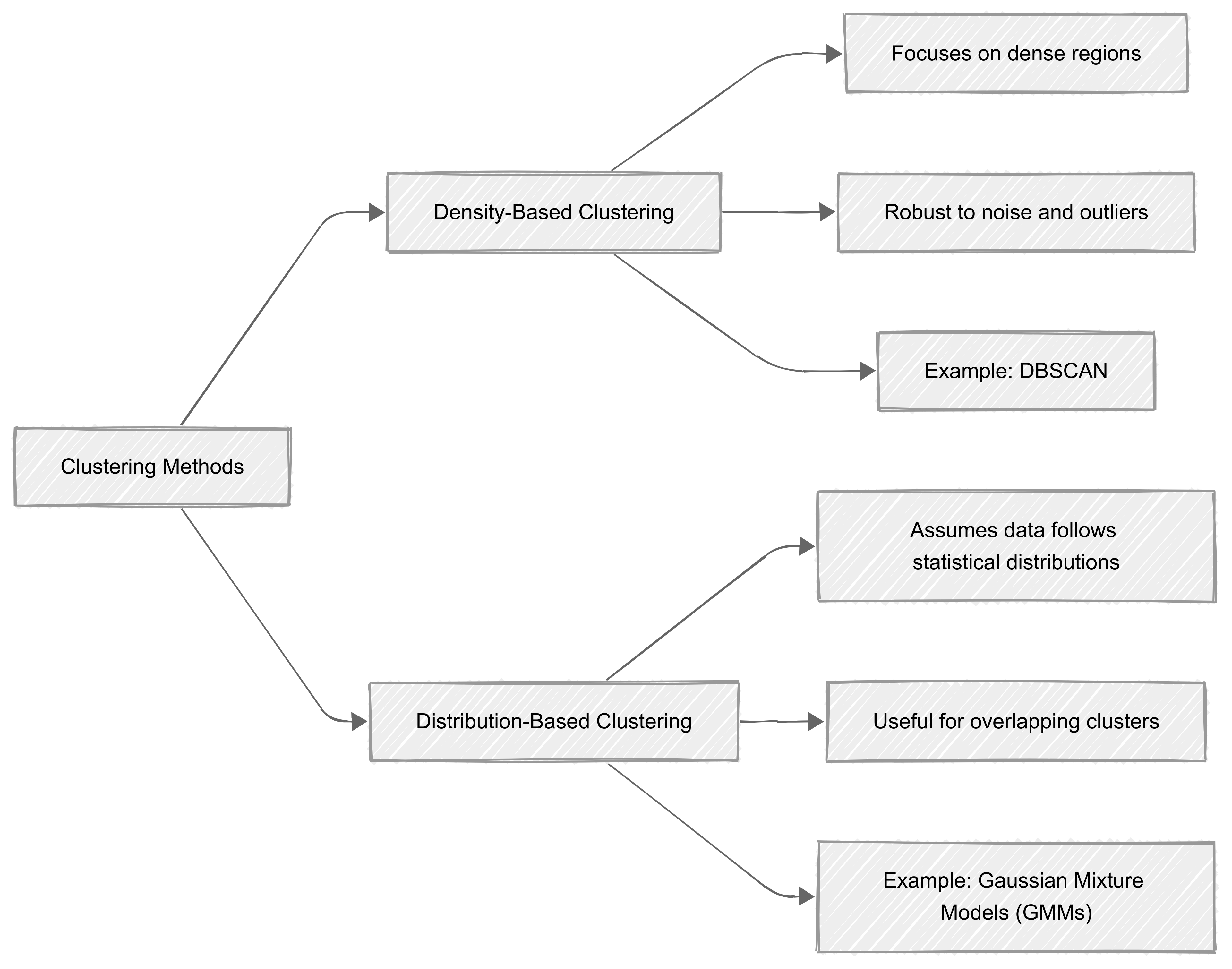
Density-based clustering

Density-based clustering focuses on identifying regions in a dataset where data points are densely packed together.

It assumes that clusters are areas of high density separated by regions of low density. This method is particularly effective when dealing with datasets that contain clusters of irregular shapes or noise (outliers).

A well-known example of a density-based algorithm is DBSCAN (Density-Based Spatial Clustering of Applications with Noise), which we’ll explore shortly. This approach works by expanding clusters from dense regions and can efficiently ignore outliers, making it robust in real-world scenarios.

Distribution-base clustering

On the other hand, distribution-based clustering assumes that data is generated from a mixture of statistical distributions, such as Gaussian distributions. It identifies clusters by estimating the underlying probability distribution of the data and assigning points to clusters based on likelihood.

One common technique is Gaussian Mixture Models (GMMs), which use probabilistic measures to determine the probability of a data point belonging to a particular cluster. This method is particularly useful when our data follows a clear probabilistic structure, or when overlapping clusters need to be analysed.

Uses

Both approaches offer unique advantages and are suited to different types of data.

Density-based clustering is really useful for complex, noisy datasets;
Distribution-based methods are ideal for data with well-defined probabilistic patterns.

5.2.3 Hard vs. soft clustering

In cluster analysis, hard clustering and soft clustering differ in how they assign data points to clusters.

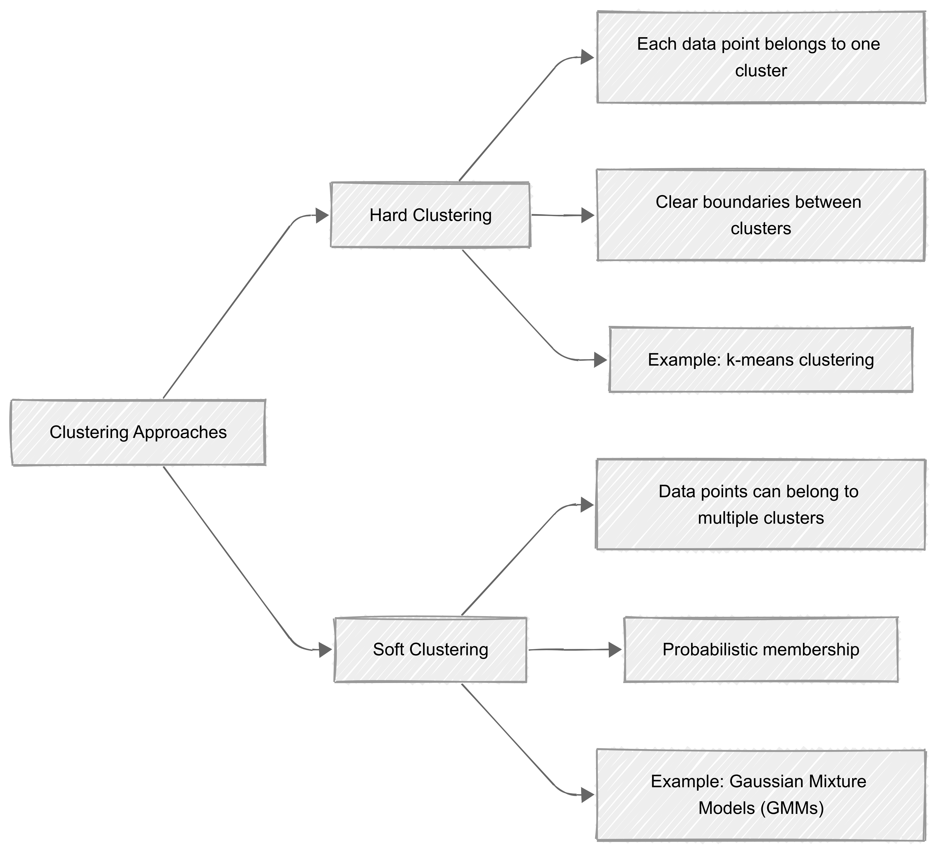
Hard clustering

‘Hard clustering’ assigns each data point to a single, well-defined cluster. In this method, every data point belongs exclusively to one group, making the boundaries between clusters clear and distinct. Algorithms like k-means clustering fall into this category.

Hard clustering is intuitive and computationally efficient, but it can struggle with datasets where clusters overlap or where there is ambiguity in cluster membership.

Soft clustering

In contrast, ‘soft clustering’ allows data points to belong to multiple clusters with varying degrees of membership. This is achieved by assigning probabilities to each point for belonging to different clusters.

For example, a data point may have a 70% likelihood of belonging to one cluster and a 30% likelihood of belonging to another. Gaussian Mixture Models (GMMs) are a common example of soft clustering algorithms.

This approach is particularly useful when the boundaries between clusters are not well-defined or when understanding the degree of association between clusters is important.

When to use

The choice between hard and soft clustering depends on the nature of your data and the problem being solved. Hard clustering is appropriate for clear-cut groups, while soft clustering is better suited for overlapping or uncertain data.

5.2.4 Feature selection and dimensionality reduction

Feature selection and dimensionality reduction are important steps in cluster analysis, as they directly impact the quality and interpretability of the clusters.

They help address issues of redundancy, noise, and high dimensionality, which can obscure meaningful patterns and lead to poor clustering performance.

Feature selection

‘Feature selection’ involves identifying the most relevant variables for clustering.

Irrelevant or redundant features (variables) can dilute the cluster structure by introducing noise or misleading similarities. In cluster analysis, unsupervised feature selection techniques like variance thresholds or spectral feature selection are often used, as no labels are available to guide the process.

Our objective is to retain features that contribute meaningfully to the inherent structure of the data.

Dimensionality reduction

‘Dimensionality reduction’ aims to transform high-dimensional data into a lower-dimensional representation while preserving as much of the relevant structure as possible.

In cluster analysis, dimensionality reduction helps by reducing computational complexity and minimizing the risk of the “curse of dimensionality,” where distances between points become less informative in high dimensions.

Popular techniques you might encounter include Principal Component Analysis (PCA), which projects data onto orthogonal components that explain the maximum variance, and t-SNE or UMAP, which are effective for visualising non-linear relationships in data. We’ll return to these later in the module.

5.3 Measuring Similarity

Measuring similarity is key to cluster analysis. Similarity quantifies how alike or different objects or datapoints are. This is crucial for tasks like recommendations, image recognition, and document clustering.

The method we use for measuring similarity depends on our data and the intended application.

Here’s an (artificial) example of a cluster analysis which minimises intra-cluster distance, and maximises inter-cluster distance:

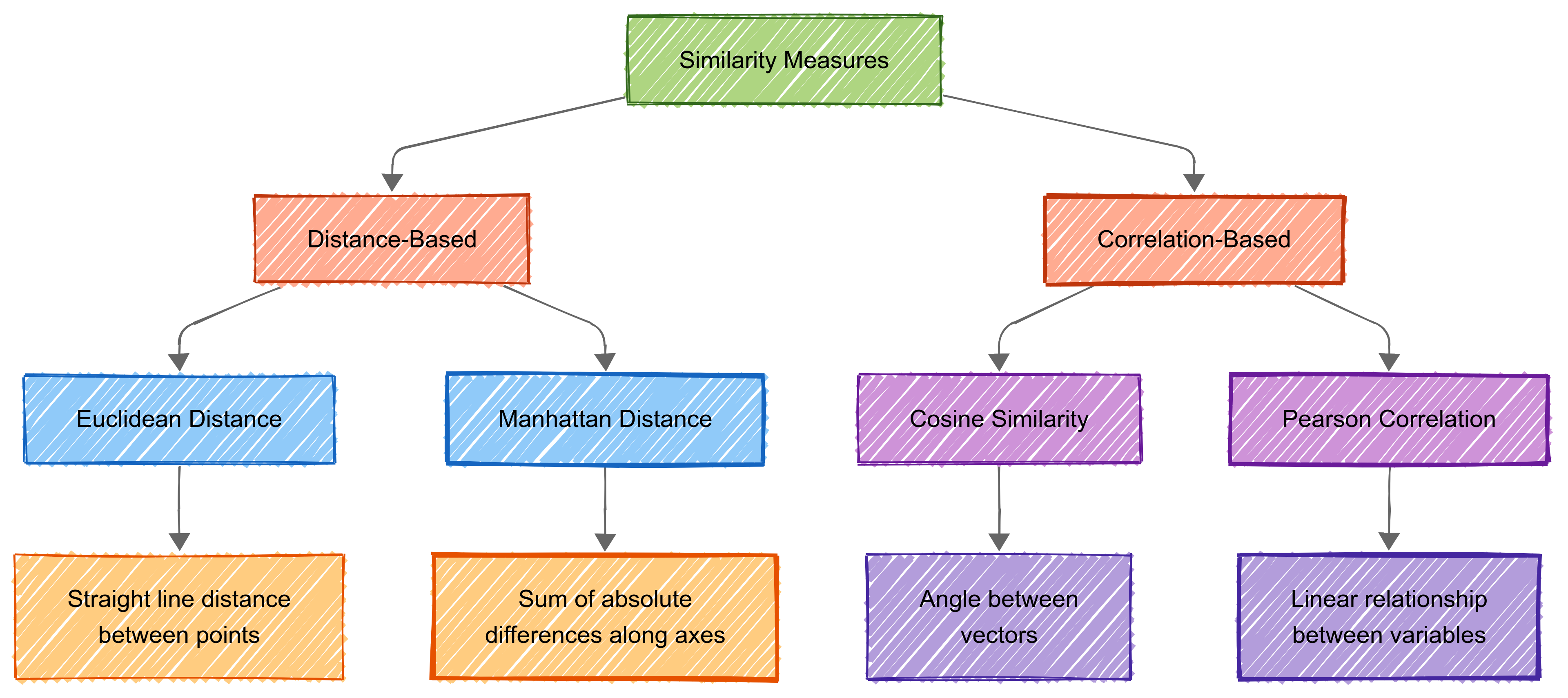
Cluster analysis uses two main types of similarly measurement:

distance-based measures (measuring how far apart items are); and
correlation-based measures (evaluating relationships between variables).

5.3.1 Euclidean distance

Euclidean distance is a measure of the straight-line distance between two points in a multidimensional space.

Euclidean distance is just the length of a straight line between two points - like measuring with a ruler. For example, if you have two points on a piece of paper, it’s the shortest possible distance you could draw between them.

Mathematically, it is the square root of the sum of squared differences between corresponding coordinates of two points.

For points $P=(p_1,p_2,…,p_n)$ and $Q=(q_1,q_2,…,q_n)$, the formula is:

\[ d(P, Q) = \sqrt{\sum_{i=1}^n (p_i - q_i)^2} \]

This distance metric is intuitive and geometrically straightforward, which makes it a common choice in many clustering algorithms.

Application in Cluster Analysis

In cluster analysis, Euclidean distance is frequently used to quantify similarity or dissimilarity between data points. Algorithms like K-means and hierarchical clustering leverage this metric to group data points into clusters.

For example, in K-means, cluster centroids are updated iteratively by minimising the Euclidean distance between data points and their assigned centroid. Similarly, hierarchical clustering builds a tree of clusters by progressively merging or splitting groups based on pairwise Euclidean distances.

Euclidean distance is most effective when our data is scaled appropriately and follows a linear structure. Standardisation or normalisation of features is often necessary to prevent variables with larger scales from dominating the distance calculations.

5.3.2 Manhattan distance

What is Manhattan Distance?

Manhattan distance, also known as ‘taxicab distance’ or $L_1-norm$, is the sum of the absolute differences between corresponding coordinates of two points.

For points $P=(p_1,p_2,…,p_n)$ and $Q=(q_1,q_2,…,q_n)$, the Manhattan distance is calculated as:

\[ d(P, Q) = \sum_{i=1}^n |p_i - q_i| \]

Unlike Euclidean distance, which measures the shortest straight-line distance, Manhattan distance reflects a grid-like path (hence its name, inspired by the Manhattan street grid).

A visual representation of Manhattan distance.

Manhattan Distance in Cluster Analysis

Manhattan distance is often used in clustering when data features are sparse, discrete, or when differences between dimensions are more meaningful when measured independently.

It’s less sensitive to outliers compared to Euclidean distance because it avoids squaring the differences. Algorithms such as K-medians or clustering methods for categorical data frequently use Manhattan distance.

In high-dimensional data, Manhattan distance can sometimes provide a better representation of similarity than Euclidean distance, especially when the features have varying distributions or are on different scales. However, like Euclidean distance, normalisation or scaling of the data (see previous topic) may still be required to avoid biasing the results toward features with larger ranges.

5.3.3 Cosine similarity

Cosine similarity is a metric that measures the cosine of the angle between two vectors in a multidimensional space.

Unlike Euclidean or Manhattan distance, cosine similarity focuses on the orientation of the vectors rather than their magnitude.

Mathematically, cosine similarity between two vectors A and B is defined as:

\[ Cosine Similarity= \cos(\theta) = \frac{A \cdot B}{\|A\| \|B\|} \]

Where:

$A⋅B$ is the dot product of vectors $A$ and $B$.
$∥A∥$ and $∥B∥$ are the magnitudes (or norms) of $A$ and $B$.

The value of cosine similarity ranges from −1 to 1, where 1 indicates identical orientation, 0 indicates orthogonality, and −1 indicates opposite directions.

Explanation

The ‘magnitude’ of a vector is a measure of its length in the vector space.

For a vector $A=(a1,a2,…,an)$, its magnitude $∥A∥$ is calculated as:

\[ ||A|| = \sqrt{a_1^2 + a_2^2 + \dots + a_n^2} \]

Application

Cosine similarity is commonly used in text and document clustering, where features represent word counts, TF-IDF scores, or other vectorised data.

Here, the magnitude of the vectors (e.g., document length) is less important than their direction (e.g., relative word frequency). Algorithms such as K-means or hierarchical clustering can be adapted to use cosine similarity instead of Euclidean distance.

Cosine similarity is particularly useful when our data is sparse or high-dimensional, as it effectively compares the relative contributions of dimensions rather than absolute differences. For instance, in text mining, cosine similarity can identify documents with similar topics even if they differ significantly in word counts.

5.3.4 Jaccard Index

The Jaccard Index (or Jaccard Similarity Coefficient) is a metric used to measure the similarity between two sets.

It’s defined as the size of the intersection of the sets divided by the size of their union.

For sets $A$ and $B$, the formula is:

\[ Jaccard Index = \frac{|A \cap B|}{|A \cup B|} \]

Where:

$∣A∩B∣$: The number of elements commo to both sets $A$ and $B$ (intersection).
$∣A∪B∣$: The total number of elements i n*either** $A$, $B$, or both (union).

The Jaccard Index ranges from 0 to 1:

0: No overlap between the sets.
1: The sets are identical.

Importance of the Jaccard Index

The Jaccard Index is widely used for comparing the similarity between finite sample sets, particularly when dealing with binary or categorical data. It’s especially useful in clustering applications where objects are represented as sets of attributes or features.

Example

Consider two sets:

$A = \{1, 2, 3, 4\}$
$B = \{3, 4, 5, 6\}$

Intersection: $A∩B=\{3,4\}$, so $∣A∩B∣=2$
Union: $A∪B=\{1,2,3,4,5,6\}$, so $∣A∪B∣=6$.

Using the formula:

\[ Jaccard Index = \frac{|A \cap B|}{|A \cup B|} = \frac{2}{6} = 0.333 \]

So, the Jaccard Index between $A$ and $B$ is 0.333, indicating a moderate level of similarity.

How does it compare with other metrics?

The Jaccard Index focuses only on the presence or absence of elements in the sets, ignoring their frequencies or magnitudes. This makes it particularly suited for applications such as:

Comparing sets of tags or categories.
Measuring overlap in clusters.
Analysing sparse data.

Applications in Cluster Analysis

In clustering, the Jaccard Index is often used to evaluate the quality of clusters or to compute pairwise similarities between objects represented as binary vectors. For example:

Binary Features: In text analysis, where documents are represented as sets of words.
Sparse Data: When datasets are dominated by 0 values, such as user-item interaction matrices.

5.4 Clustering Algorithms

5.4.1 Introduction

Clustering algorithms, which are central to cluster analysis, help identify natural groupings within our data. They analyse patterns and similarities between data points to organise them into meaningful clusters.

The core principle behind clustering is to maximise similarity within groups while maximising differences between groups. This allows for the discovery of inherent structures in data without pre-existing labels.

There are a number of different algorithms that are commonly used for cluster analysis, including:

K-means clustering
Hierarchical clustering
DBSCAN
Gaussian Mixture models

5.4.2 k-means clustering

Introduction

K-means is widely used in clustering due to its simplicity and efficiency. The algorithm begins by initialising k centroids, where k is the number of clusters defined by the user.

These centroids are placed randomly within the data space. Each data point is then assigned to the cluster represented by the nearest centroid, with the distance typically measured using the Euclidean distance formula.

After all points have been assigned, the centroids of the clusters are updated to the mean position of all points within each cluster. This process of assignment and update is repeated iteratively until the centroids stabilise, meaning they no longer change significantly, or a maximum number of iterations is reached.

Example

Consider performance data for players on a football team, which might include metrics such as goals scored, assists, tackles, and distance covered during a game.

K-means can group these players into clusters that represent different playing styles, such as strikers, midfielders, and defenders, based on their performance characteristics.

How does it work?

The algorithm begins by randomly initialising k centroids in the data space.

Each data point $x_i$ is assigned to the cluster $C_j$ whose centroid $μ_j$ is closest to it, typically based on the Euclidean distance.

The assignment step minimises the following distance:

\[ d(x_i, \mu_j) = \sqrt{\sum_{m=1}^n (x_{im} - \mu_{jm})^2} \]

After the assignment, the centroids are updated by taking the mean of all data points in the cluster:

\[ u_j = \frac{1}{|C_j|} \sum_{x_i \in C_j} x_i \]

This process of assignment and update is repeated iteratively until the centroids stabilise ,or a maximum number of iterations is reached.

5.4.3 Hierarchical clustering

Unlike k-means clustering (which is a partitioning model), hierarchical clustering builds nested clusters in a hierarchical tree structure, either from the bottom up (agglomerative) or the top down (divisive).

In the agglomerative approach, each data point starts as its own cluster. The algorithm identifies the two closest clusters based on a distance metric, such as single-linkage or complete-linkage, and merges them into a single cluster. This merging process is repeated iteratively until all data points form one single cluster.

In the divisive approach, the process starts with all data points in a single cluster, which is recursively split until each data point is its own cluster. The final output is a dendrogram, a tree-like diagram that represents the hierarchical structure of the clusters.

Example

In sport, hierarchical clustering could be used to analyse football team performances across multiple matches. Metrics such as possession percentages, shots on target, and goal differences could reveal clusters of teams with similar performance profiles.

The dendrogram might show clusters of elite teams, mid-level teams, and underperforming teams.

How does it work?

Hierarchical clustering creates nested clusters organised into a tree-like structure, either from the bottom up (agglomerative) or the top down (divisive).

In the agglomerative approach, each data point initially forms its own cluster. At each step, the two clusters with the smallest distance are merged.

The distance between two clusters A and B can be defined in several ways, such as single-linkage (minimum distance), complete-linkage (maximum distance), or average-linkage:

\[ Single-linkage: d(A, B) = \min_{x \in A, y \in B} \|x - y\| \]

\[ Complete-linkage: d(A, B) = \max_{x \in A, y \in B} \|x - y\| \]

\[ Average-linkage: d(A, B) = \frac{1}{|A||B|} \sum_{x \in A} \sum_{y \in B} \|x - y\| \]

This merging continues until all data points are grouped into one cluster, forming a dendrogram. Divisive clustering works in the opposite direction, starting with one large cluster and recursively splitting it.

The dendrogram

5.4.4 DBSCAN

Introduction

DBSCAN is a density-based clustering algorithm that identifies clusters based on the density of data points in a given region.

The algorithm classifies points into three categories: core points, border points, and noise.

A core point is a data point that has at least a specified number of neighbouring points (MinPts) within a given radius (eps).
Border points are those that are within the neighbourhood of a core point but do not themselves have enough neighbours to be core points
Points that do not fall into these two categories are considered noise.

DBSCAN starts by identifying core points and expanding clusters around them by including neighbouring points. The process continues until no more points can be added to any cluster. DBSCAN is particularly effective for identifying clusters of varying shapes and handling noise in the data.

How does it work?

Each point in the dataset is classified as a core point, border point, or noise based on two parameters: the radius ϵ and the minimum number of points MinPts within that radius.

A core point is one that has at least $MinPts$ neighbours within a radius $ϵ$.

Border points are those that fall within the ϵ-neighbourhood of a core point but have fewer than $MinPts$ neighbours. Any point that is neither a core nor a border point is classified as noise.

The algorithm starts by identifying core points and expanding clusters around them by including neighboring points within $ϵ$. This process continues until no more points can be added to any cluster.

Mathematically, a point $p$ is considered part of a cluster if:

\[ |p - q\| \leq \epsilon \quad \text{and} \quad |\{q : \|p - q\| \leq \epsilon\}| \geq \text{MinPts} \]

DBSCAN is particularly useful for identifying clusters of arbitrary shapes and handling noise in the data.

We will cover DBSCAN in more detail in Chapter 21.

5.4.5 Gaussian Mixture Models

Gaussian Mixture Models (GMMs) are a probabilistic approach to cluster analysis.

Unlike methods like K-means, which assign each data point to a single cluster, GMMs assume that data points are generated from a mixture of multiple Gaussian distributions.

This probabilistic framework allows for more flexibility in capturing complex cluster shapes and assigning a probability of belonging to each cluster for every data point.

Gaussian Mixture Models (GMM) assume that our data comes from several groups (or clusters), each shaped like a 3D bell curve, called a Gaussian distribution.

The components of a Gaussian Mixture

Every cluster in GMM is defined by three things:

Mean ($μk$) (‘mew’): This is the centre of the cluster. Think of it as the average position of the data points in that group.
Covariance ($Σk$): This describes the shape and size of the cluster. It tells us how spread out the points are and in which direction they vary.
Mixing Coefficient (**$πk$): This is how much weight each cluster contributes to the overall dataset. For example, if 60% of the data comes from one group and 40% from another, the weights would be 0.6 and 0.4. All the weights add up to 1.

The probability of a data point

For each cluster, GMM uses a mathematical formula to calculate the probability that a point belongs to that cluster. This formula is called the Gaussian (or Normal) Distribution.

In simple terms, it describes how data is spread out around the mean.

For a data point x in cluster k, the probability is:

\[ \mathcal{N}(x | \mu_k, \Sigma_k) = \frac{1}{\sqrt{(2\pi)^d |\Sigma_k|}} \exp\left(-\frac{1}{2}(x - \mu_k)^T \Sigma_k^{-1} (x - \mu_k)\right) \]

Here’s what each part means:

$μk$: The centre of the cluster.
$Σk$: The shape and spread of the cluster.
$d$: The number of features in our data (e.g., height, weight, speed in sports data).
$exp()$: Exponential function that ensures probabilities are between 0 and 1.

Assigning points to clusters (E-Step)

Instead of hard assignments (like K-means), GMM uses soft assignments.

For each data point, it calculates the probability of belonging to every cluster.

These probabilities are called responsibilities and are written as $γik$, meaning the responsibility of cluster k for point i.

The formula for $γik$ is:

\[ γ_{ik} = \frac{\pi_k \cdot \mathcal{N}(x_i | \mu_k, \Sigma_k)}{\sum_{j=1}^K \pi_j \cdot \mathcal{N}(x_i | \mu_j, \Sigma_j)} \]

The numerator $(πk⋅N)$ gives the probability for cluster k.
The denominator is the sum of probabilities for all clusters, ensuring the total probability is 1.

For example, if a footballer has a 70% chance of being a striker and 30% of being a midfielder, their responsibilities for the two clusters are 0.7 and 0.3.

Updating the cluster parameters (M-Step)

Once responsibilities are calculated, the algorithm updates the parameters of each cluster to better fit the data.

Here’s how:

New Mean ($μk$): The mean is updated as the weighted average of all points, where the weights are the responsibilities:

\[ u_k = \frac{\sum_{i=1}^N \gamma_{ik} x_i}{\sum_{i=1}^N \gamma_{ik}} \]

This ensures the center of the cluster moves closer to the points it’s responsible for.

New Covariance ($Σk$): The covariance is updated to reflect the spread of points within the cluster:

\[ \sum k = \frac{\sum_{i=1}^N \gamma_{ik} (x_i - \mu_k)(x_i - \mu_k)^T}{\sum_{i=1}^N \gamma_{ik}} \]

This helps reshape the cluster to better fit the data.
New Mixing Coefficient ($πk$): The weight for each cluster is updated to reflect the proportion of points assigned to it:

\[ \pi_k = \frac{\sum_{i=1}^N \gamma_{ik}}{N} \]

Iterating until convergence

The algorithm alternates between calculating responsibilities (E-step) and updating parameters (M-step) until the parameters stop changing significantly.

This is called convergence. At the end, each cluster is defined by its updated mean, covariance, and mixing coefficient.

We will cover GMMs in greater detail in Chapter 21.

5.5 Validating Clusters

Finally, cluster validation helps assess the quality and reliability of clustering results, regardless of what method or methods have been used to create the clusters.

At its core, it involves evaluating how well a clustering algorithm has performed in grouping similar data points together while keeping dissimilar points in different clusters.

We’ve covered several different algorithms that can be used for clustering. Validation helps us check and compare how these algorithms have performed.

Various metrics and indices have been developed to quantify the effectiveness of clustering solutions.

These validation measures typically focus on two main aspects:

internal validation (which examines the clustering structure using only the data itself)
external validation (which compares clustering results against known class labels when available).

5.5.1 Silhouette Score

The silhouette score is a metric commonly used to evaluate the quality of clustering by measuring how similar each point is to its own cluster compared to other clusters.

A high silhouette score suggests that clusters are compact and well-separated from each other.

The score ranges from -1 to 1, where a high value indicates that the point is well-matched to its own cluster and poorly matched to neighbouring clusters.

The calculation of the silhouette score involves two distances: the mean intra-cluster distance (a) and the mean nearest-cluster distance ($b$) for each sample. The silhouette score $S$ for each point is computed as:

\[ S = \frac{b - a}{\max(a, b)} \]

5.5.2 Davies-Bouldin Index

The Davies-Bouldin Index (DBI) is another method for validating the clustering configuration.

It’s based on a ratio between the within-cluster scatter and the between-cluster separation.

A lower DBI value indicates a model with better separation between the clusters. The index is calculated as follows:

\[ DBI = \frac{1}{k} \sum_{i=1}^k \max_{j \neq i} \left(\frac{s_i + s_j}{d_{ij}}\right) \]

where $s_i$ is the average distance of all points in the cluster to their centroid, $d_{ij}$ is the distance between centroids of clusters $i$ and $j$, and $k$ is the number of clusters.

5.5.3 Calinksi-Harabasz Index

The Calinski-Harabasz Index (CH Index) is another method for evaluating the quality of clustering

It is also known as the ‘Variance Ratio Criterion’, and it compares the dispersion between clusters with the dispersion within clusters.

Higher values generally indicate better-defined clustering because the clusters are more distinct from each other.

\[ CH = \frac{\text{Tr}(B_k) \cdot (N - k)}{\text{Tr}(W_k) \cdot (k - 1)} \]

Where:

$Tr(B_k$) is the trace of the between-cluster dispersion matrix,
$Tr(W_k)$ is the trace of the within-cluster dispersion matrix,
$N$ is the total number of points,
$k$ is the number of clusters.

5.5.4 Dunn Index

Finally. the Dunn Index is another measure used to validate the quality of cluster configurations.

It evaluates clustering by identifying compact and well-separated clusters.

The Dunn Index is defined as the ratio of the smallest distance between observations in different clusters to the largest intra-cluster distance.

The goal is to maximise the Dunn Index, where higher values indicate better clustering with greater separation between clusters and compactness within clusters.

\[ DI = \min_{1 \leq i \leq k} \left( \min_{1 \leq j \leq k, i \neq j} \left( \frac{\delta(i, j)}{\max_{1 \leq l \leq k} \Delta(l)} \right) \right) \]

Where:

$δ(i, j)$ (‘delta i j’) is the distance between clusters $i$ and $j$, typically measured as the distance between the nearest members of the clusters.
$Δ(l)$ is the maximum intra-cluster distance in cluster $l$.