# Load required libraries
library(tseries)
Registered S3 method overwritten by 'quantmod':
method from
as.zoo.data.frame zoo library(forecast)
library(ggplot2)This practical will guide you through identifying and handling stationarity issues in a time series dataset.
You will:
# Load required libraries
library(tseries)Registered S3 method overwritten by 'quantmod':
method from
as.zoo.data.frame zoo library(forecast)
library(ggplot2)Objective: Generate a synthetic time series that exhibits non-stationary behavior.
set.seed(123)
time_series <- ts(cumsum(rnorm(100)), frequency = 12, start = c(2000, 1))Objective: Plot the time series to visually inspect trends or seasonality.
Before applying any tests, a visual inspection can often reveal key patterns.
Look for:
plot(time_series, main='Original Time Series', ylab='Value', xlab='Time')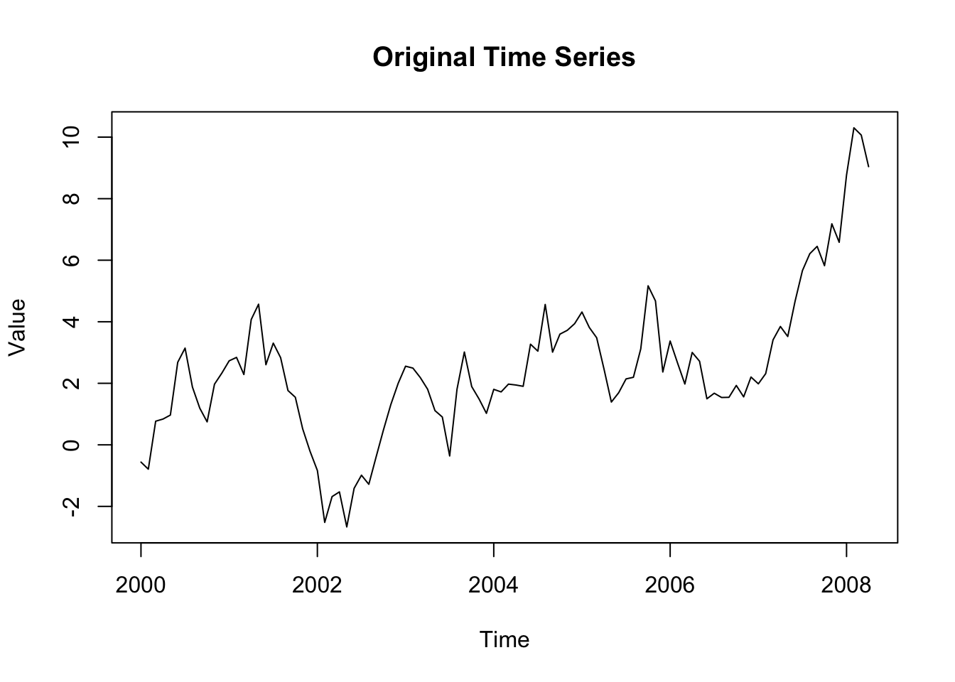
Objective: Use the Augmented Dickey-Fuller (ADF) test to check for stationarity.
The ADF test helps determine whether a series is stationary by testing the null hypothesis (H0) that a unit root is present.
adf_test_result <- adf.test(time_series)
adf_test_result
    Augmented Dickey-Fuller Test

data:  time_series
Dickey-Fuller = -1.8871, Lag order = 4, p-value = 0.6234
alternative hypothesis: stationaryObjective: If the series is non-stationary, apply first differencing and plot it.
Differencing removes trends by subtracting the previous value from the current value. This should stabilise the mean and make the series stationary.
diff_series <- diff(time_series)
plot(diff_series, main='Differenced Time Series', ylab='Differenced Value', xlab='Time')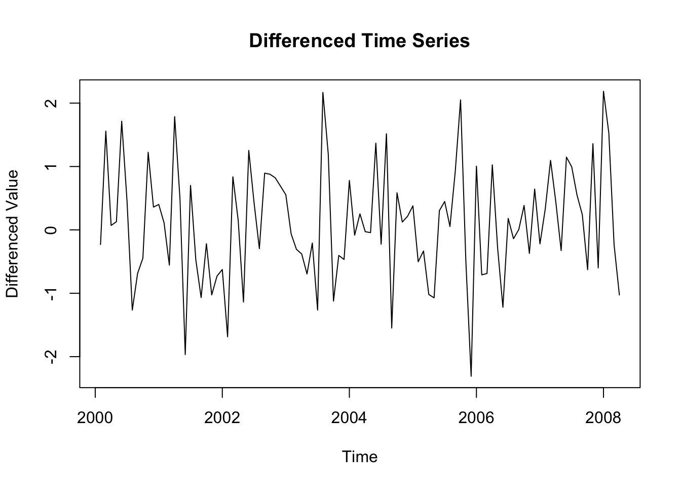
Objective: Check if differencing has made the series stationary.
Now that we have applied differencing, we re-run the ADF test.
If the p-value is now < 0.05, the series is likely stationary.
If it is still > 0.05, further transformations may be needed.
adf.test(na.omit(diff_series))Warning in adf.test(na.omit(diff_series)): p-value smaller than printed p-value
    Augmented Dickey-Fuller Test

data:  na.omit(diff_series)
Dickey-Fuller = -4.5735, Lag order = 4, p-value = 0.01
alternative hypothesis: stationaryObjective: Log transformation stabilises variance if there are large fluctuations.
Some time series exhibit increasing variability over time. A log transformation can help by compressing larger values and expanding smaller ones, making variance more consistent.
if (any(time_series <= 0)) {
  log_series <- log(time_series - min(time_series) + 1)  # Shift to avoid log(0) or negative values
} else {
  log_series <- log(time_series)
}

plot(log_series, main='Log Transformed Time Series', ylab='Log Value', xlab='Time')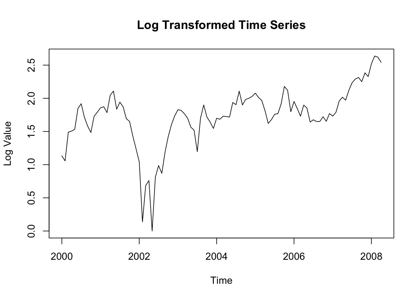
Objective: Combine transformations to achieve stationarity if needed.
If differencing alone was not enough, we can try applying both log transformation and differencing together. This is useful when data exhibits both trend and variance instability.
log_diff_series <- diff(log_series)
log_diff_series <- na.omit(log_diff_series)  # Remove NA values
plot(log_diff_series, main='Log-Differenced Time Series', ylab='Value', xlab='Time')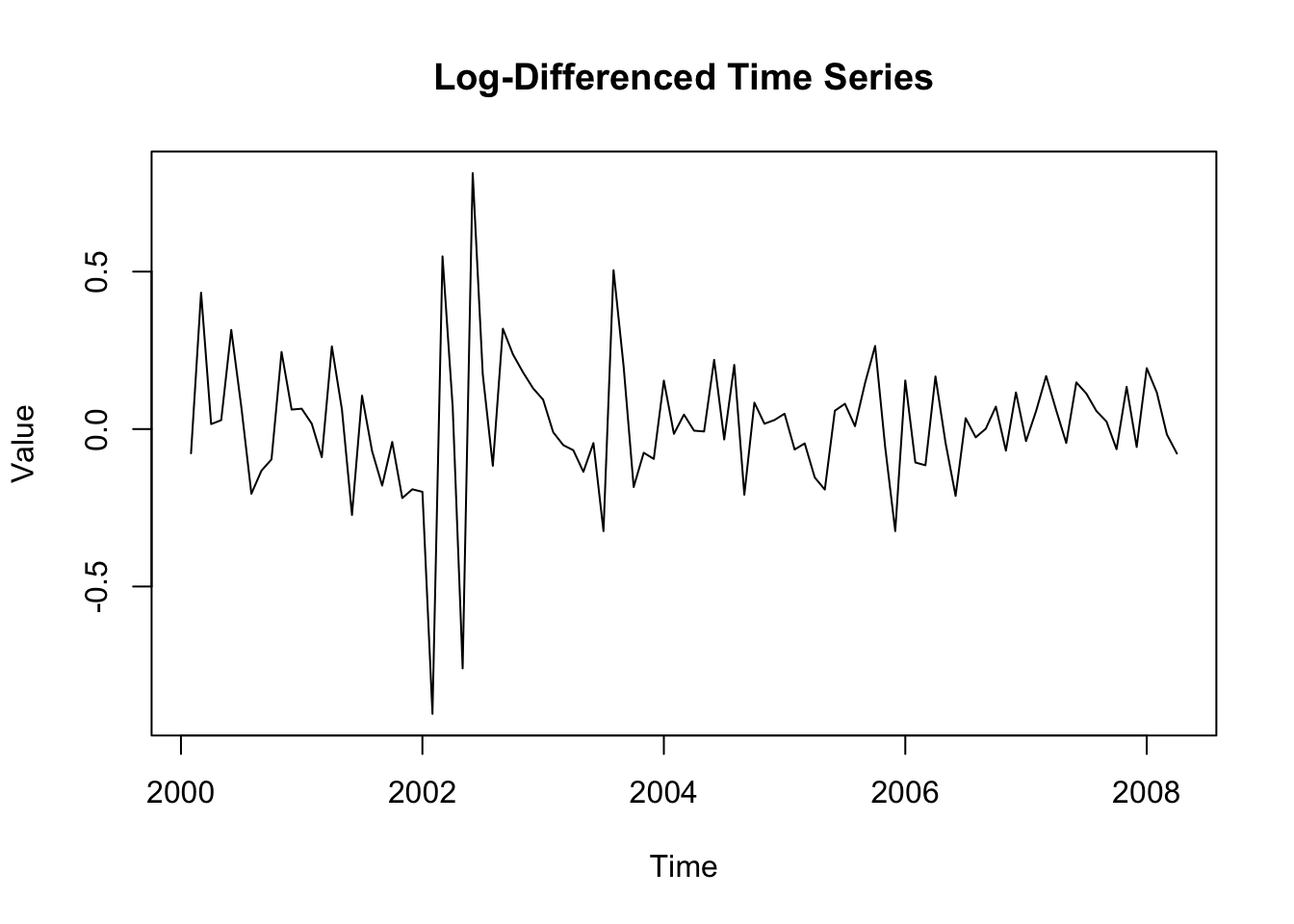
Objective: Confirm that the final transformation has achieved stationarity.
The final check ensures that all necessary transformations have been applied successfully. If the p-value is < 0.05, the series is now stationary and suitable for further analysis.
adf.test(log_diff_series)
    Augmented Dickey-Fuller Test

data:  log_diff_series
Dickey-Fuller = -3.9228, Lag order = 4, p-value = 0.01585
alternative hypothesis: stationaryObjective: Reflect on the effectiveness of transformations.
Consider the following questions: