Seasonal and Panel Data Models - Practical

Introduction

In this practical, I’ll demonstrate how to apply seasonal and panel data approaches to TSA in R.

Visualising and decomposing seasonal patterns

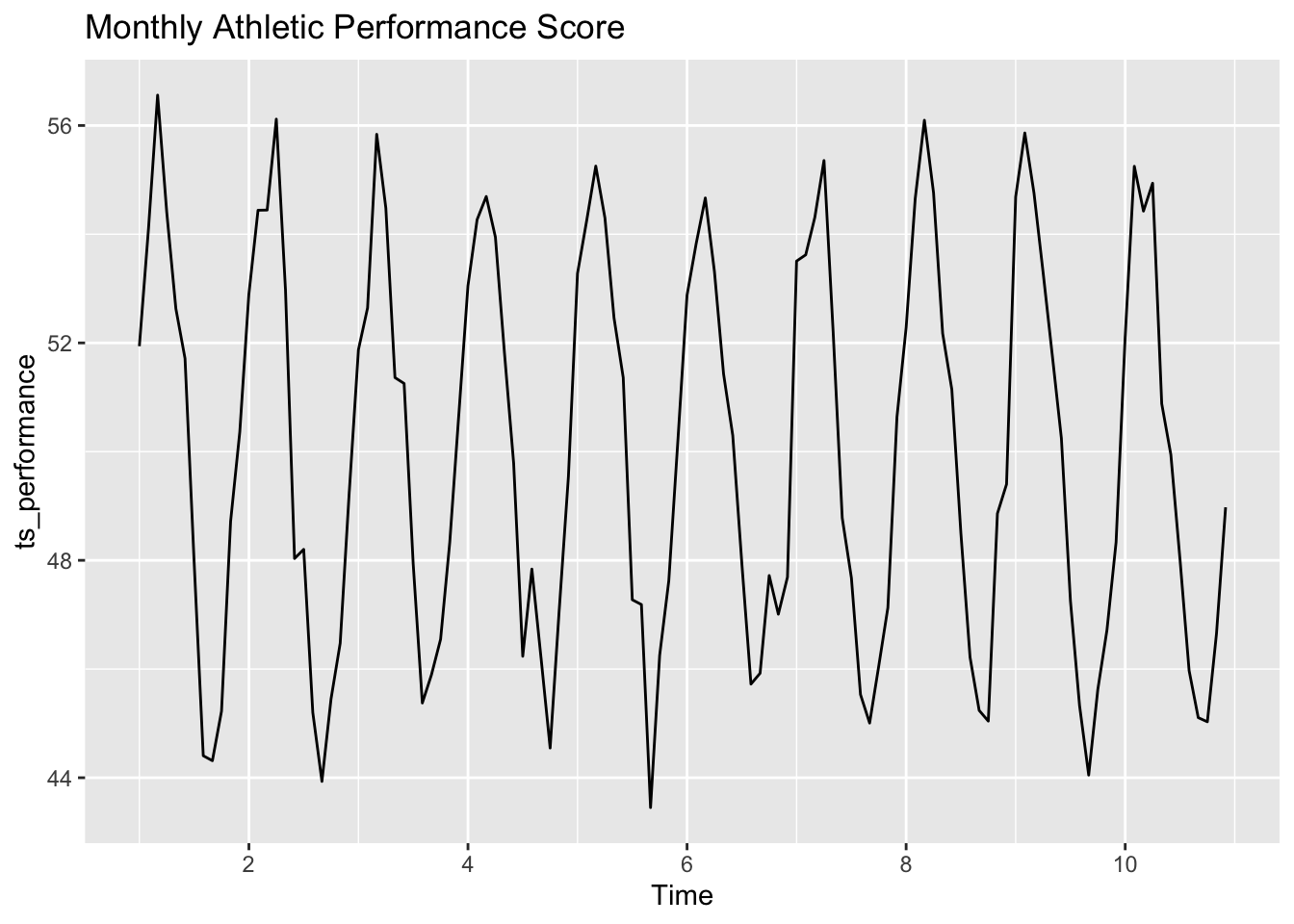
Question: “How does an athlete’s performance score vary seasonally over the training and competition cycle?”

Analysis

In athletics, performance can fluctuate over the year due to training cycles/ peaking for major events/ recovery periods.

This code simulates a monthly performance score series (higher is better) with seasonal peaks (perhaps representing better performance in the summer months) and random variation:

Code

library(ggplot2)
library(forecast)

Registered S3 method overwritten by 'quantmod':
  method            from
  as.zoo.data.frame zoo

Code

set.seed(123)
time <- 1:120

# Simulate a seasonal pattern (e.g., peak performance during summer months)
seasonality <- 5 * sin(2 * pi * time / 12)
noise <- rnorm(120, mean = 0, sd = 1)
performance <- 50 + seasonality + noise  # Base performance score with seasonal variation
ts_performance <- ts(performance, frequency = 12)
autoplot(ts_performance) + ggtitle("Monthly Athletic Performance Score")

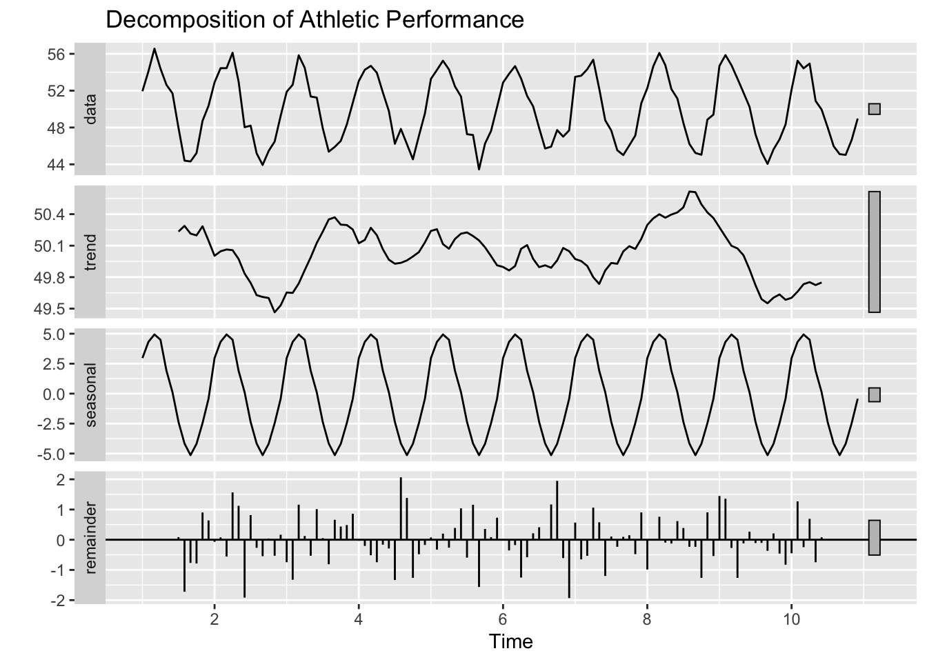
Decomposition

Decomposition helps answer:

“What parts of the performance trend are driven by seasonality versus long-term improvements or random factors?”

Code

decomposed <- decompose(ts_performance)
autoplot(decomposed) + ggtitle("Decomposition of Athletic Performance")

Interpretation

Trend: Could reflect gradual improvement from training over several years.
Seasonality: Highlights cyclical peaks (e.g., performance boosts during competition season).
Noise: Random fluctuations due to day-to-day conditions.

Forecast Opportunity

After decomposing, we can forecast future performance by modeling the seasonal component separately.

This might help coaches schedule training to maintain peak performance during competitions.

Code

library(ggplot2)
library(forecast)

set.seed(123)
time <- 1:120

# Simulate performance data with a seasonal pattern (e.g., peak during competition months)
seasonality <- 5 * sin(2 * pi * time / 12)
noise <- rnorm(120, mean = 0, sd = 1)
performance <- 50 + seasonality + noise
ts_performance <- ts(performance, frequency = 12)

# Decompose time series
decomposed <- decompose(ts_performance)
autoplot(decomposed) + ggtitle("Decomposition of Athletic Performance")

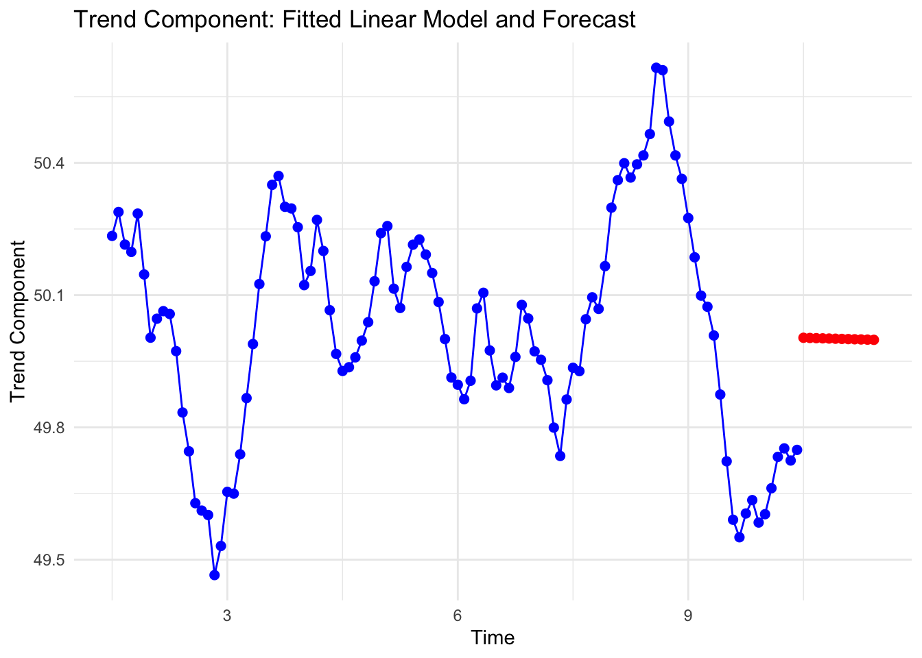
Since the seasonal pattern is assumed to repeat, we focus on forecasting the underlying trend.

Here, we extract the trend component (ignoring the edge NAs) and fit a simple linear model.

Code

trend <- decomposed$trend
time_idx <- time(ts_performance)
valid <- !is.na(trend)
trend_clean <- trend[valid]
time_clean <- time_idx[valid]

# Fit linear model to trend component
trend_model <- lm(trend_clean ~ time_clean)
summary(trend_model)


Call:
lm(formula = trend_clean ~ time_clean)

Residuals:
     Min       1Q   Median       3Q      Max 
-0.57727 -0.13959  0.01491  0.17777  0.60262 

Coefficients:
             Estimate Std. Error t value Pr(>|t|)    
(Intercept) 50.056757   0.061689 811.436   <2e-16 ***
time_clean  -0.005097   0.009491  -0.537    0.592    
---
Signif. codes:  0 '***' 0.001 '**' 0.01 '*' 0.05 '.' 0.1 ' ' 1

Residual standard error: 0.2562 on 106 degrees of freedom
Multiple R-squared:  0.002714,  Adjusted R-squared:  -0.006694 
F-statistic: 0.2885 on 1 and 106 DF,  p-value: 0.5923

Code

# Forecast trend for next 12 months
future_time <- seq(max(time_clean) + 1/12, by = 1/12, length.out = 12)
trend_forecast <- predict(trend_model, newdata = data.frame(time_clean = future_time))


# Create data frames for plotting
df_trend <- data.frame(time = time_clean, trend = trend_clean)
df_forecast <- data.frame(time = future_time, trend = trend_forecast)

# Visualise trend, fitted line, forecast
library(ggplot2)
ggplot() +
  geom_point(data = df_trend, aes(x = time, y = trend), color = "blue", size = 2) +
  geom_line(data = df_trend, aes(x = time, y = trend), color = "blue") +
  geom_line(data = df_forecast, aes(x = time, y = trend), color = "red", linetype = "dashed") +
  geom_point(data = df_forecast, aes(x = time, y = trend), color = "red", size = 2) +
  labs(title = "Trend Component: Fitted Linear Model and Forecast",
       x = "Time",
       y = "Trend Component") +
  theme_minimal()

Extract seasonal pattern

The seasonal component from the decomposition provides the repeating pattern. Since our data has a frequency of 12, we extract the seasonal indices for one complete cycle (i.e., 12 months).

# Extract the seasonal pattern (first full cycle)
seasonal_pattern <- decomposed$seasonal[1:12]

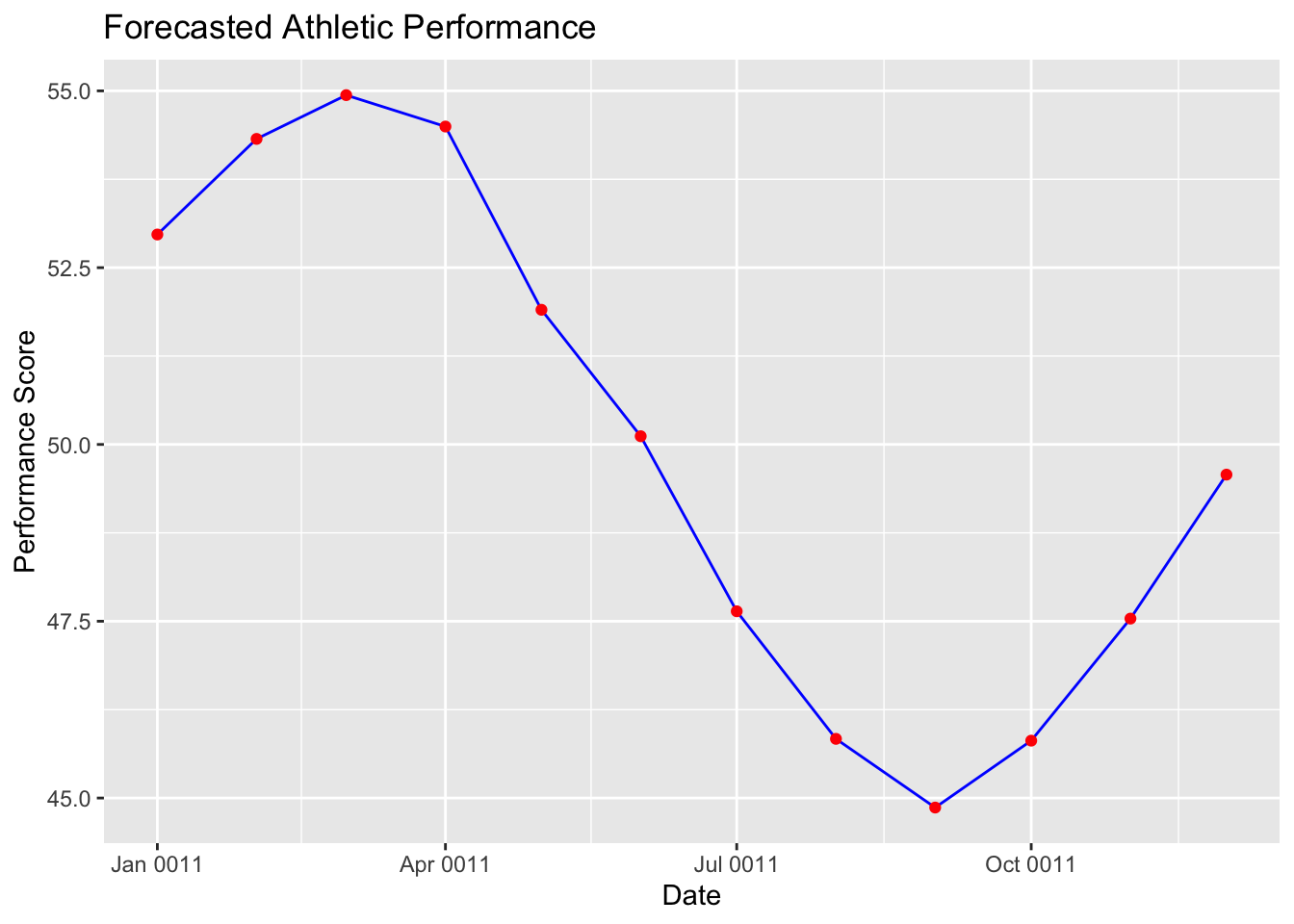
Combine trend and seasonal forecasts

Assuming the residuals average to zero, the forecast for future performance is the sum of the forecasted trend and the known seasonal pattern.

Code

# Since frequency is 12, we take the first 12 months as the seasonal pattern
seasonal_pattern <- decomposed$seasonal[1:12]

forecast_performance <- trend_forecast + seasonal_pattern

end_info <- end(ts_performance)  # returns c(last_year, last_period)
end_year <- end_info[1]
end_period <- end_info[2]

if(end_period == frequency(ts_performance)) {
  start_year <- end_year + 1
  start_month <- 1
} else {
  start_year <- end_year
  start_month <- end_period + 1
}

start_date <- as.Date(sprintf("%d-%02d-01", start_year, start_month))
future_dates <- seq(start_date, by = "month", length.out = 12)

# Create a data frame with forecast dates and values
forecast_df <- data.frame(Date = future_dates, Forecast = forecast_performance)

# Plot forecast
ggplot(forecast_df, aes(x = Date, y = Forecast)) +
  geom_line(color = "blue") +
  geom_point(color = "red") +
  ggtitle("Forecasted Athletic Performance") +
  xlab("Date") +
  ylab("Performance Score")

Seasonal Regression & SARIMA Modeling

Question: “Can we quantify how much each month affects performance, and forecast future performance using seasonal models?”

Seasonal regression

A regression model with monthly dummy variables can help answer, for instance: “How much better is performance in July compared to January?”

# Create a data frame with a date sequence representing months
dates <- seq(as.Date("2020-01-01"), by = "month", length.out = 120)
performance_df <- data.frame(Date = dates, Performance = as.numeric(ts_performance))
performance_df$Month <- factor(format(performance_df$Date, "%m"))

# Fit a regression model with monthly dummies
seasonal_model <- lm(Performance ~ Month, data = performance_df)
summary(seasonal_model)


Call:
lm(formula = Performance ~ Month, data = performance_df)

Residuals:
     Min       1Q   Median       3Q      Max 
-2.22621 -0.55895 -0.02099  0.54204  1.97031 

Coefficients:
            Estimate Std. Error t value Pr(>|t|)    
(Intercept)  52.8521     0.2835 186.442  < 2e-16 ***
Month02       1.4401     0.4009   3.592 0.000495 ***
Month03       2.2531     0.4009   5.620 1.50e-07 ***
Month04       1.6406     0.4009   4.092 8.26e-05 ***
Month05      -0.8780     0.4009  -2.190 0.030659 *  
Month06      -2.5925     0.4009  -6.467 2.99e-09 ***
Month07      -5.1528     0.4009 -12.853  < 2e-16 ***
Month08      -6.9754     0.4009 -17.399  < 2e-16 ***
Month09      -7.9401     0.4009 -19.806  < 2e-16 ***
Month10      -7.1025     0.4009 -17.716  < 2e-16 ***
Month11      -5.3916     0.4009 -13.449  < 2e-16 ***
Month12      -3.3409     0.4009  -8.334 2.73e-13 ***
---
Signif. codes:  0 '***' 0.001 '**' 0.01 '*' 0.05 '.' 0.1 ' ' 1

Residual standard error: 0.8964 on 108 degrees of freedom
Multiple R-squared:  0.9452,    Adjusted R-squared:  0.9396 
F-statistic: 169.4 on 11 and 108 DF,  p-value: < 2.2e-16

Interpretation:

The coefficients for each month indicate the average deviation from the baseline month, which could help athletic staff understand seasonal effects.

SARIMA Forecasting

To capture both autoregressive behavior and seasonality in the performance data, a SARIMA model can be used.

For example, if you’re forecasting an athlete’s future performance to plan training cycles:

sarima_model <- auto.arima(ts_performance, seasonal = TRUE)
summary(sarima_model)

Series: ts_performance 
ARIMA(0,0,0)(0,1,2)[12] 

Coefficients:
         sma1    sma2
      -1.0450  0.1803
s.e.   0.1534  0.1146

sigma^2 = 0.8686:  log likelihood = -154.03
AIC=314.07   AICc=314.3   BIC=322.11

Training set error measures:
                      ME      RMSE       MAE        MPE     MAPE    MASE
Training set -0.03598833 0.8759365 0.6619653 -0.0873729 1.332821 0.59219
                   ACF1
Training set 0.04221482

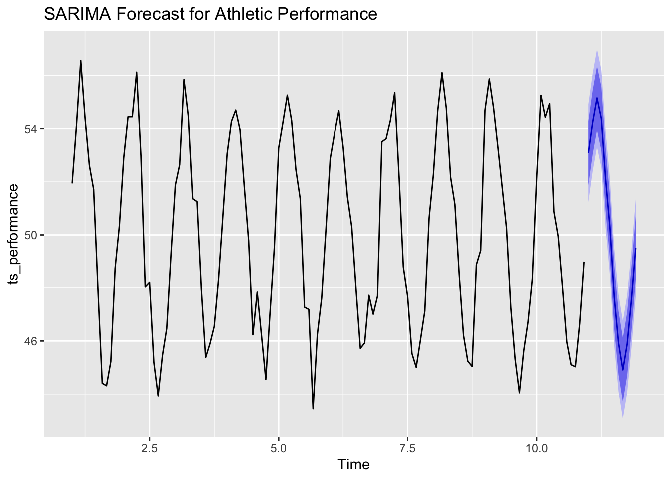
forecast_sarima <- forecast(sarima_model, h = 12)
autoplot(forecast_sarima) + ggtitle("SARIMA Forecast for Athletic Performance")

Interpretation:

The forecast shows predicted performance scores along with confidence intervals that reflect seasonal peaks and valleys.

Advanced Diagnostics

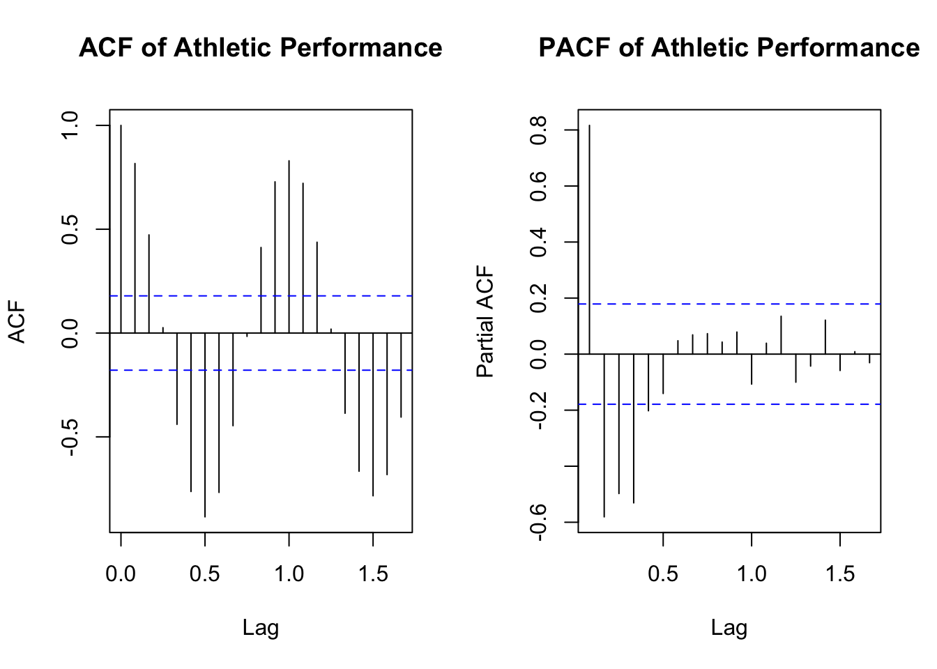
Use ACF/PACF plots and residual checks to ensure the model is properly capturing the underlying patterns:

par(mfrow = c(1,2))
acf(ts_performance, main = "ACF of Athletic Performance")
pacf(ts_performance, main = "PACF of Athletic Performance")

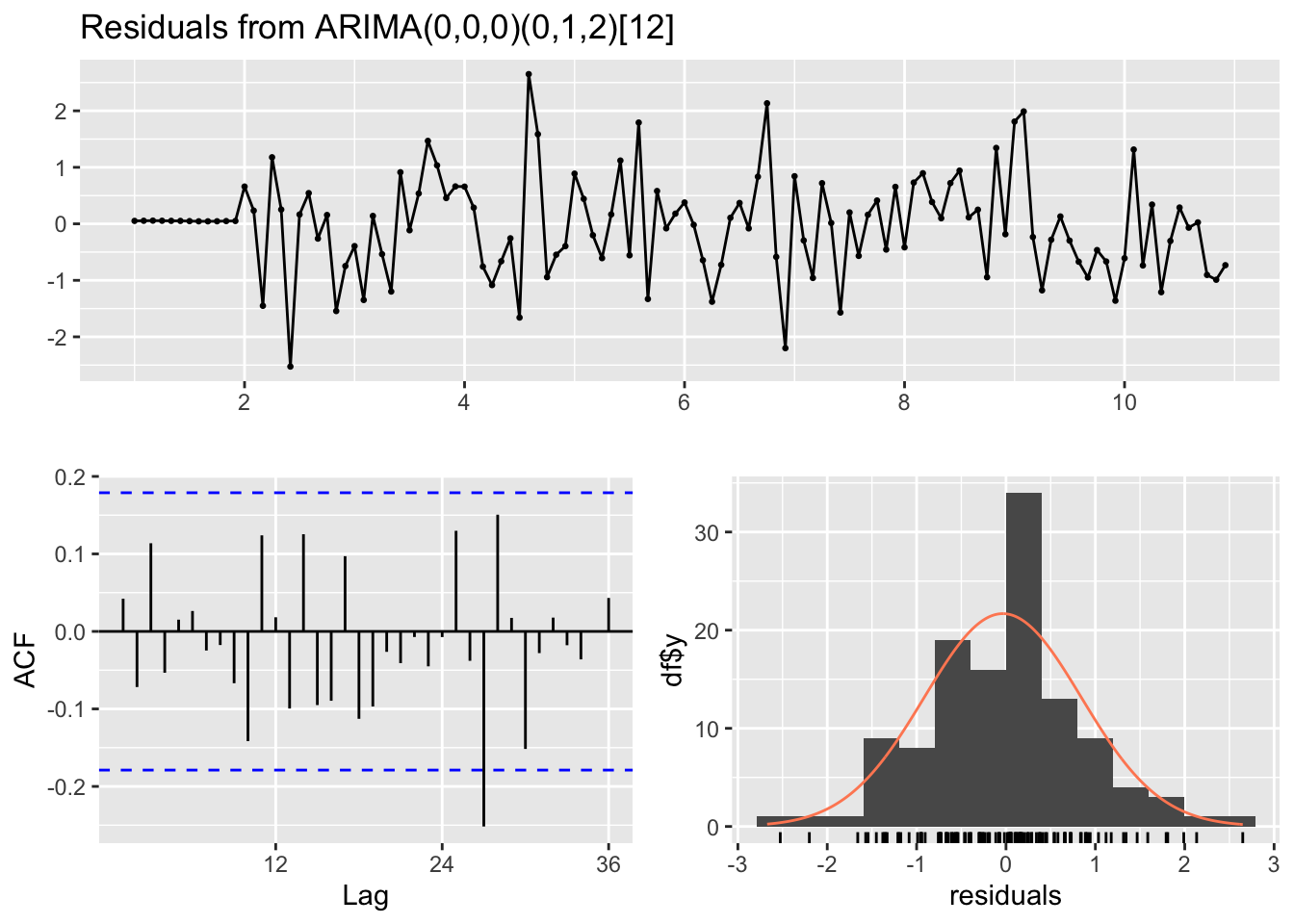
par(mfrow = c(1,1))

checkresiduals(sarima_model)


    Ljung-Box test

data:  Residuals from ARIMA(0,0,0)(0,1,2)[12]
Q* = 19.543, df = 22, p-value = 0.6116

Model df: 2.   Total lags used: 24

Interpretation:

Residual diagnostics help verify that the model has removed any serial correlation, ensuring reliable forecasts.

Panel Data Models: Multiple Athletes Across Competitions

Question: “How do individual differences among athletes affect performance across multiple competitions, and which athletes are expected to improve?”

Imagine you’re tracking performance scores for 10 athletes over 5 competitions.

The following code simulates such panel data, where each athlete has a unique baseline and each competition introduces its own effect:

library(plm)
library(dplyr)


Attaching package: 'dplyr'

The following objects are masked from 'package:plm':

    between, lag, lead

The following objects are masked from 'package:stats':

    filter, lag

The following objects are masked from 'package:base':

    intersect, setdiff, setequal, union

set.seed(123)
n_athletes <- 10    # 10 athletes
n_competitions <- 5 # 5 competitions

# Create panel data
athlete <- factor(rep(1:n_athletes, each = n_competitions))
competition <- rep(1:n_competitions, times = n_athletes)
# Simulate athlete-specific effects and competition-specific effects
athlete_effect <- rep(rnorm(n_athletes, mean = 5, sd = 1), each = n_competitions)
competition_effect <- rep(rnorm(n_competitions, mean = 0, sd = 1), times = n_athletes)
error <- rnorm(n_athletes * n_competitions, mean = 0, sd = 2)
performance_score <- 50 + 0.8 * competition + athlete_effect + competition_effect + error

# Combine into a data frame
panel_data <- data.frame(athlete, competition, performance_score)
head(panel_data)

  athlete competition performance_score
1       1           1          60.03743
2       1           2          57.39504
3       1           3          53.30706
4       1           4          59.15292
5       1           5          56.93810
6       2           1          54.65826

Estimating fixed and random effects models

To control for unobserved, athlete-specific characteristics that might affect performance:

# Fixed Effects (FE) model: controls for athlete-specific factors
fe_model <- plm(performance_score ~ competition, 
                data = panel_data, 
                index = c("athlete", "competition"), 
                model = "within")

# Random Effects (RE) model: assumes athlete effects are random
re_model <- plm(performance_score ~ competition, 
                data = panel_data, 
                index = c("athlete", "competition"), 
                model = "random")

# Compare models using the Hausman test
library(lmtest)

Loading required package: zoo


Attaching package: 'zoo'

The following objects are masked from 'package:base':

    as.Date, as.Date.numeric

phtest(fe_model, re_model)


    Hausman Test

data:  performance_score ~ competition
chisq = 8.7715e-15, df = 4, p-value = 1
alternative hypothesis: one model is inconsistent

Interpretation:

A significant Hausman test suggests that the FE model is more appropriate, meaning that individual athlete differences are correlated with competition effects.
If RE is acceptable, you can generalise findings across a broader population of athletes.

Forecasting with Panel Data

Panel data models can be used to forecast an athlete’s performance in future competitions.

For instance, to forecast for the next competition (e.g., competition 6), you might extend the trend from your model.

Here’s a simple illustration using the FE model:

library(plm)
library(dplyr)

# Estimate the Random Effects (RE) model
re_model <- plm(performance_score ~ competition, 
                data = panel_data, 
                index = c("athlete", "competition"), 
                model = "random")

# Extract overall coefficients from the RE model
model_coef <- coef(re_model)
overall_intercept <- model_coef["(Intercept)"]
beta_re <- model_coef["competition"]

# 1. Population-Level (or New Athlete) Forecast for Competition 6:
population_forecast <- overall_intercept + beta_re * 6
cat("Population-level forecast for Competition 6:", population_forecast, "\n")

Population-level forecast for Competition 6: NA

# 2. Individual Athlete Forecasts using their random effects:
# Extract random effects for each athlete as a named vector
re_effects_vec <- as.vector(ranef(re_model))
athlete_names <- names(ranef(re_model))
re_effects_df <- data.frame(athlete = athlete_names, 
                            random_effect = re_effects_vec)

# For each athlete: Forecast = overall_intercept + beta_re * 6 + athlete's random effect
individual_forecasts <- re_effects_df %>%
  mutate(Forecast = overall_intercept + beta_re * 6 + random_effect)

print(individual_forecasts)

   athlete random_effect Forecast
1        1   -0.20196725       NA
2        2   -0.92080159       NA
3        3    0.68342027       NA
4        4    0.59546048       NA
5        5    0.15289934       NA
6        6    1.14605455       NA
7        7   -0.05111622       NA
8        8   -0.41070505       NA
9        9   -0.19571145       NA
10      10   -0.79753307       NA

Forecast Opportunity:

The random effect represents the estimated deviation of each athlete from the overall (population-level) baseline performance.

In other words, it quantifies how much better or worse an athlete performs relative to the average athlete once the common factors (like the overall intercept and the effect of competition) have been accounted for.

Beyond ARIMA: Hybrid & Combined Approaches in Athletics

Question: “How can we combine seasonal decomposition with athlete panel data to forecast performance trends across the season?”

Hybrid Approaches

For instance, if you have panel data where each athlete’s monthly performance exhibits seasonality, you can:

Step 1: Decompose each athlete’s performance series using methods like STL (Seasonal-Trend Decomposition). Step 2: Extract the trend components and model them using panel regression to control for athlete-specific factors. Step 3: Combine the forecasted trend with the average seasonal pattern to predict future performance. This combined method leverages the clarity of seasonal decomposition with the robustness of panel data analysis, offering nuanced insights into performance management.

# Load required libraries
library(dplyr)
library(tidyr)
library(purrr)
library(ggplot2)
library(forecast)
library(plm)

set.seed(123)
n_athletes <- 10
n_months <- 36  # Data for 36 months

# Simulate monthly performance:
# - Each athlete has a unique effect
# - Global trend over time
# - Seasonal component (periodic, with period 12)
# - Random noise
athlete <- factor(rep(1:n_athletes, each = n_months))
month <- rep(1:n_months, times = n_athletes)
athlete_effect <- rep(rnorm(n_athletes, mean = 0, sd = 3), each = n_months)
trend_component <- 0.2 * month              # Global trend component
seasonal_component <- 5 * sin(2 * pi * month/12)  # Seasonal pattern
noise <- rnorm(n_athletes * n_months, 0, 2)
performance <- 50 + athlete_effect + trend_component + seasonal_component + noise

data <- data.frame(athlete = athlete, month = month, performance = performance)
head(data)

  athlete month performance
1       1     1    53.46674
2       1     2    53.76833
3       1     3    54.72012
4       1     4    53.67007
5       1     5    50.70689
6       1     6    53.09240

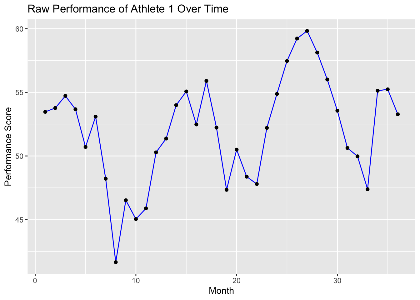
# Plot Raw Performance for a Single Athlete
# visualise raw performance of athlete 1 over time.
data %>% 
  filter(athlete == "1") %>% 
  ggplot(aes(x = month, y = performance)) +
  geom_line(color = "blue") +
  geom_point() +
  ggtitle("Raw Performance of Athlete 1 Over Time") +
  xlab("Month") + ylab("Performance Score")

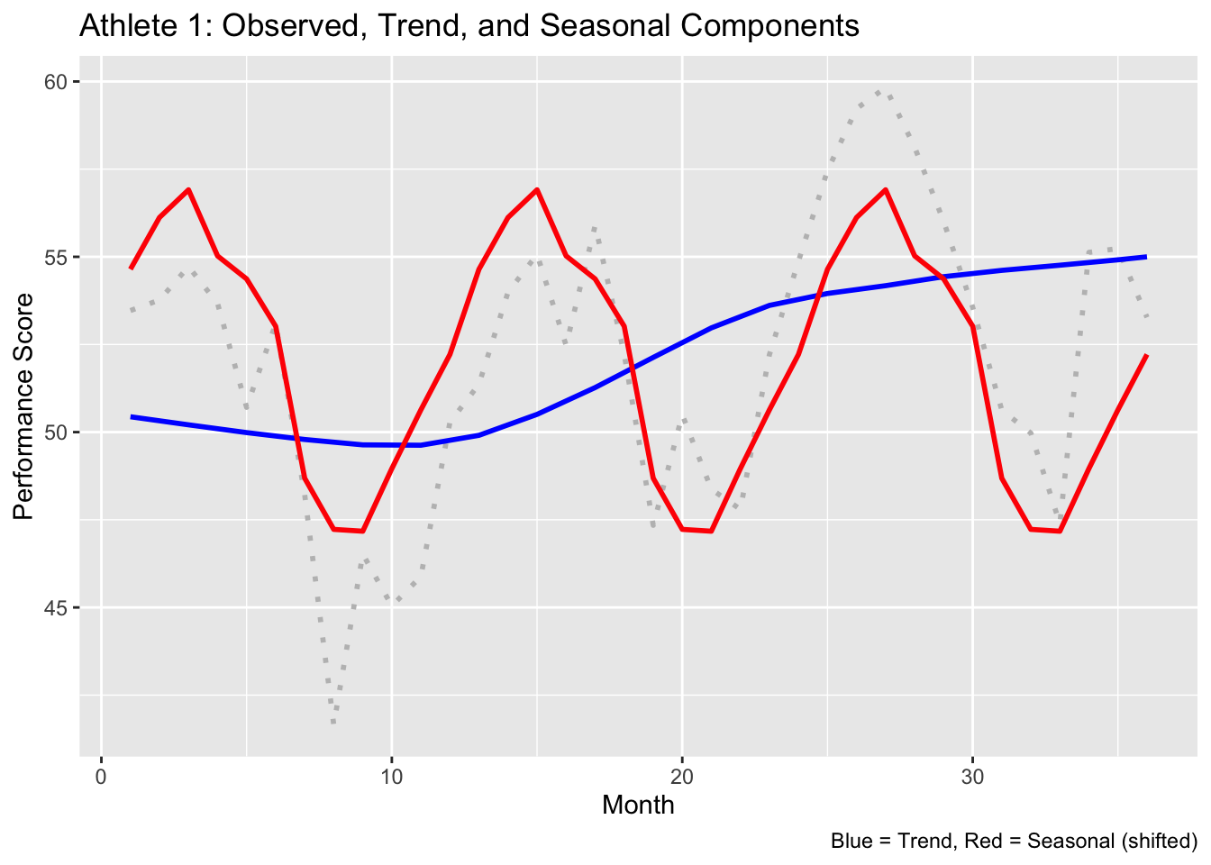
# Seasonal Decomposition (STL)
# Nest data by athlete - each athlete's performance series can be decomposed individually.
data_nested <- data %>%
  group_by(athlete) %>%
  nest()

# For each athlete, create a time series object (with frequency 12) and perform STL decomposition.
# Then immediately extract the trend and seasonal components.
data_nested <- data_nested %>%
  mutate(ts_obj = map(data, ~ ts(.x$performance, frequency = 12)),
         stl_decomp = map(ts_obj, ~ stl(.x, s.window = "periodic")),
         trend = map(stl_decomp, ~ as.numeric(.x$time.series[, "trend"])),
         seasonal = map(stl_decomp, ~ as.numeric(.x$time.series[, "seasonal"]))) %>%
  # Remove the raw time series and STL objects to simplify later steps.
  select(-ts_obj, -stl_decomp)

# Visualisation: Decomposition for Athlete 1
# Extract data for athlete 1 and create a data frame for plotting.
athlete1 <- data_nested %>% filter(athlete == "1")
athlete1_decomp <- data.frame(
  month = 1:n_months,
  trend = athlete1$trend[[1]],
  seasonal = athlete1$seasonal[[1]],
  observed = data %>% filter(athlete == "1") %>% pull(performance)
)

# Plot observed performance, trend, and seasonal components
ggplot(athlete1_decomp, aes(x = month)) +
  geom_line(aes(y = observed), color = "gray", size = 1, linetype = "dotted") +
  geom_line(aes(y = trend), color = "blue", size = 1) +
  geom_line(aes(y = seasonal + mean(observed)), color = "red", size = 1) +
  ggtitle("Athlete 1: Observed, Trend, and Seasonal Components") +
  xlab("Month") +
  ylab("Performance Score") +
  labs(caption = "Blue = Trend, Red = Seasonal (shifted)")

Warning: Using `size` aesthetic for lines was deprecated in ggplot2 3.4.0.
ℹ Please use `linewidth` instead.

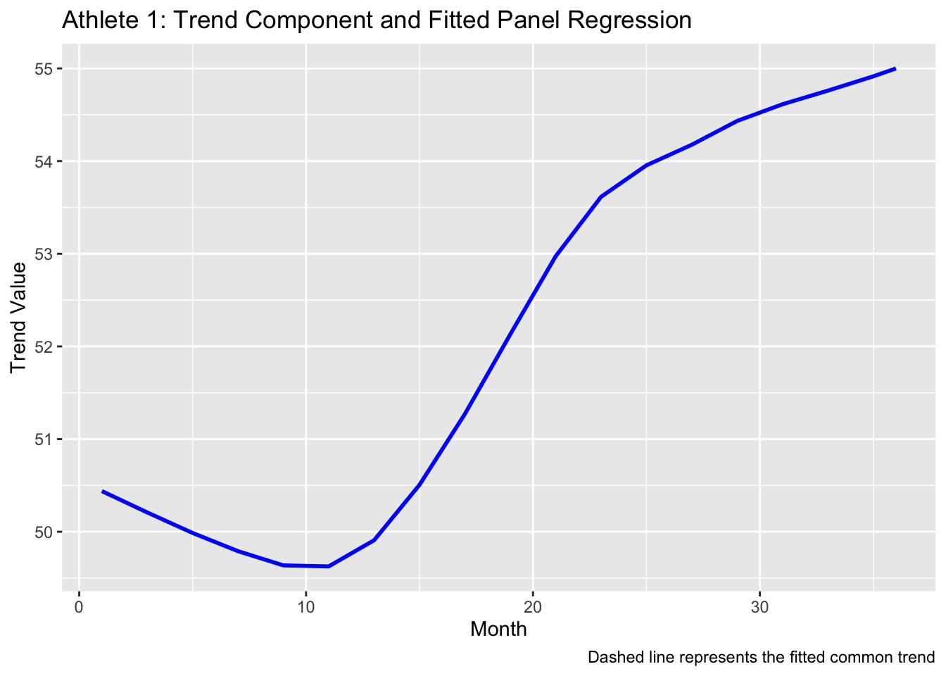
# Modeling Trend Component via Panel Regression
# Unnest trend values along with a month index for each athlete.
trend_data <- data_nested %>%
  select(athlete, trend) %>%
  mutate(month = list(1:n_months)) %>%   # Create a month index for each athlete
  unnest(cols = c(month, trend)) %>%
  rename(trend_value = trend)

# Run a panel regression (pooled model) on the extracted trend component.
trend_panel <- plm(trend_value ~ month, data = trend_data, index = c("athlete", "month"), model = "pooling")
summary(trend_panel)

Pooling Model

Call:
plm(formula = trend_value ~ month, data = trend_data, model = "pooling", 
    index = c("athlete", "month"))

Balanced Panel: n = 10, T = 36, N = 360

Residuals:
    Min.  1st Qu.   Median  3rd Qu.     Max. 
-4.03631 -1.90874 -0.70118  0.86232  5.46133 

Coefficients:
            Estimate Std. Error t-value  Pr(>|t|)    
(Intercept) 50.84521    0.88289 57.5893 < 2.2e-16 ***
month2       0.15698    1.24860  0.1257 0.9000266    
month3       0.31396    1.24860  0.2515 0.8016237    
month4       0.47676    1.24860  0.3818 0.7028356    
month5       0.63955    1.24860  0.5122 0.6088506    
month6       0.80919    1.24860  0.6481 0.5173942    
month7       0.97883    1.24860  0.7839 0.4336478    
month8       1.15120    1.24860  0.9220 0.3572178    
month9       1.32357    1.24860  1.0600 0.2899126    
month10      1.49490    1.24860  1.1973 0.2320811    
month11      1.66622    1.24860  1.3345 0.1829872    
month12      1.83820    1.24860  1.4722 0.1419349    
month13      2.01018    1.24860  1.6100 0.1083825    
month14      2.20373    1.24860  1.7650 0.0785119 .  
month15      2.39728    1.24860  1.9200 0.0557386 .  
month16      2.58595    1.24860  2.0711 0.0391427 *  
month17      2.77462    1.24860  2.2222 0.0269611 *  
month18      2.94269    1.24860  2.3568 0.0190284 *  
month19      3.11076    1.24860  2.4914 0.0132240 *  
month20      3.28946    1.24860  2.6345 0.0088303 ** 
month21      3.46816    1.24860  2.7776 0.0057944 ** 
month22      3.69433    1.24860  2.9588 0.0033160 ** 
month23      3.92049    1.24860  3.1399 0.0018456 ** 
month24      4.16682    1.24860  3.3372 0.0009447 ***
month25      4.41314    1.24860  3.5345 0.0004680 ***
month26      4.64255    1.24860  3.7182 0.0002364 ***
month27      4.87195    1.24860  3.9019 0.0001161 ***
month28      5.05435    1.24860  4.0480 6.466e-05 ***
month29      5.23675    1.24860  4.1941 3.540e-05 ***
month30      5.40540    1.24860  4.3292 1.997e-05 ***
month31      5.57405    1.24860  4.4642 1.111e-05 ***
month32      5.73786    1.24860  4.5954 6.195e-06 ***
month33      5.90168    1.24860  4.7266 3.409e-06 ***
month34      6.05890    1.24860  4.8526 1.897e-06 ***
month35      6.21612    1.24860  4.9785 1.043e-06 ***
month36      6.36713    1.24860  5.0994 5.808e-07 ***
---
Signif. codes:  0 '***' 0.001 '**' 0.01 '*' 0.05 '.' 0.1 ' ' 1

Total Sum of Squares:    3906.3
Residual Sum of Squares: 2525.6
R-Squared:      0.35346
Adj. R-Squared: 0.28362
F-statistic: 5.06092 on 35 and 324 DF, p-value: 7.0748e-16

# Plot Trend Component with Fitted Panel Regression
# overlay fitted trend line (which is common across athletes) for athlete 1.
beta_est <- coef(trend_panel)["month"]
intercept_est <- coef(trend_panel)["(Intercept)"]
trend_data_athlete1 <- trend_data %>% filter(athlete == "1")
trend_data_athlete1 <- trend_data_athlete1 %>%
  mutate(fitted = intercept_est + beta_est * month)

ggplot(trend_data_athlete1, aes(x = month)) +
  geom_line(aes(y = trend_value), color = "blue", size = 1) +
  geom_line(aes(y = fitted), color = "darkgreen", size = 1, linetype = "dashed") +
  ggtitle("Athlete 1: Trend Component and Fitted Panel Regression") +
  xlab("Month") +
  ylab("Trend Value") +
  labs(caption = "Dashed line represents the fitted common trend")

Warning: Removed 36 rows containing missing values or values outside the scale range
(`geom_line()`).

# Forecast trend for a future period (e.g., month 37)
trend_forecast_value <- intercept_est + beta_est * 37

# Extracting Average Seasonal Pattern
# Unnest seasonal values with their corresponding month index.
seasonal_data <- data_nested %>%
  select(athlete, seasonal) %>%
  mutate(month = list(1:n_months)) %>%
  unnest(cols = c(month, seasonal)) %>%
  # Compute the cycle month (1 to 12)
  mutate(cycle_month = ((month - 1) %% 12) + 1)

# Compute  average seasonal effect for each cycle month.
avg_seasonal <- seasonal_data %>%
  group_by(cycle_month) %>%
  summarise(avg_seasonal = mean(seasonal))
print(avg_seasonal)

# A tibble: 12 × 2
   cycle_month avg_seasonal
         <dbl>        <dbl>
 1           1        2.00 
 2           2        3.86 
 3           3        4.59 
 4           4        3.90 
 5           5        2.32 
 6           6       -0.146
 7           7       -2.41 
 8           8       -4.15 
 9           9       -4.31 
10          10       -4.11 
11          11       -1.85 
12          12        0.318

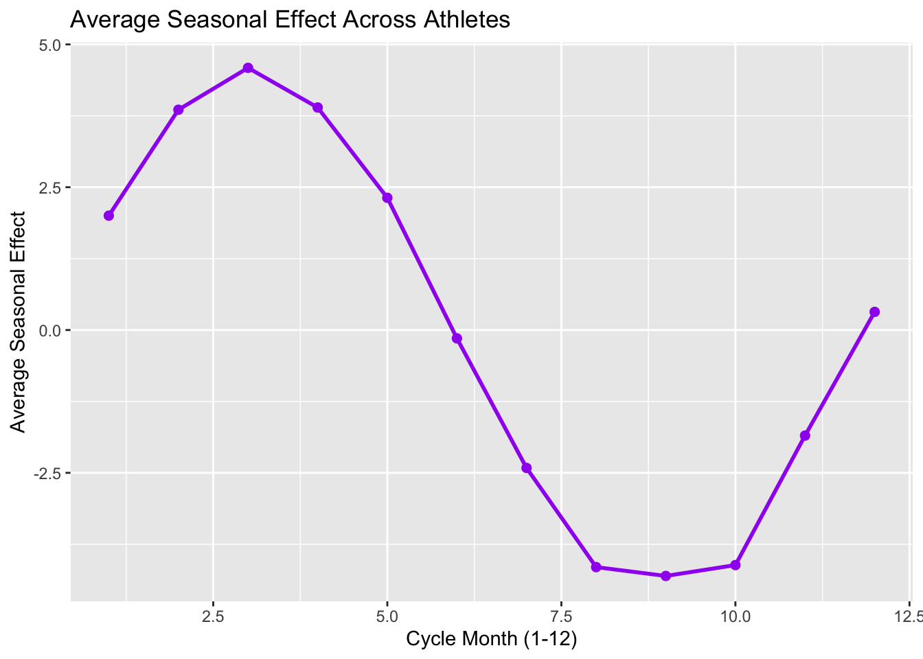
#  Plot the Average Seasonal Pattern
ggplot(avg_seasonal, aes(x = cycle_month, y = avg_seasonal)) +
  geom_line(color = "purple", size = 1) +
  geom_point(color = "purple", size = 2) +
  ggtitle("Average Seasonal Effect Across Athletes") +
  xlab("Cycle Month (1-12)") +
  ylab("Average Seasonal Effect")

# For forecasting month 37, determine its cycle month.
forecast_cycle_month <- ((37 - 1) %% 12) + 1  # For month 37, cycle_month will be 1
seasonal_forecast_value <- avg_seasonal %>%
  filter(cycle_month == forecast_cycle_month) %>%
  pull(avg_seasonal)

# Final combined forecast
# The final forecast for month 37 is sum of forecasted trend and seasonal effect.
final_forecast <- trend_forecast_value + seasonal_forecast_value
cat("Forecasted performance for month 37:", final_forecast, "\n")

Forecasted performance for month 37: NA