Only move on to this section when you have finished the previous reading.
4.1 Learning Outcomes
By the end of this section, you should:
understand how variables and and assignment operators are used in R
be confident in using the different data types within R
understand the use of vectors in R, and performing basic vector operations
4.2 Variables and Assignment
In programming, variables are objects (containers) in which we store data values and store the results of calculations or other operations on existing data. When you create a variable, there is nothing in it until you put something in it!
‘Assignment operators’ allow you to place values into variables.
Assignment Operators
We use assignment operators to put things into variables.
There are three assignment operators in R: <-, -> and =.
Of these, <-is the most frequently used.
<- can be used to assign a value to a variable, as in the following example:
num <-42# assigns the value 42 to a variable 'num'# note: this command actually does two things. It create a variable called 'num', and puts the value 42 into 'num'.print(num) # prints the value of 'num' to the console
[1] 42
num <-56# we've now replaced the value of 42 with 56print(num) # prints the new value of 'num' to the console
[1] 56
Note that, in the previous lines of code, we used several important commands within R that you should be familiar with:
In R, the hash symbol # is used to comment lines of code. In these early examples I will comment frequently on the code. This is to help you understand exactly what is going on.
Later, I’ll restrict my comments to what is necessary, which is similar to what we would do in the ‘real world’.
Important
Please remember to include meaningful comments in any scripts you create during your MSc programme. It’s essential that other people can understand how your code works, and comments are a great way to do this.
The print command is used to return a value to our console window, so we can check what is happening in our code. This is especially useful when writing new code, as it helps you keep an eye on how your code is working.
In the last example, we put numbers into our variable [num].
The <- operator can also be used to assign a character or character string to a variable (this can be a letter, or a piece of text):
greeting <-"hello world"# assigns the value 'hello world' to variable 'greeting'print(greeting) # print the value of 'greeting' to the console
[1] "hello world"
It can also be used to assign a logical value to a variable:
win <-TRUE# assign the value TRUE to the variable 'win'.print(win) # print the value of 'win' to the console
[1] TRUE
We’ll cover the different kinds of variables in R below (Section 4.3).
Performing operations with variables
The <- assignment operator can also be used to perform arithmetical calculations:
# define two variables, x and yx <-10y <-3# perform some arithmetic operations on those variablessum <- x + y # adds the values of each variable. note that this creates another variable that is the SUM of the variables x and y.difference <- x - y # subtracts the values of y from xproduct <- x * y # the product is the outcome when we multiplyquotient <- x / y # the quotient is the outcome when we divide# print the results to the console windowprint(sum) # print the variable sum to the console
[1] 13
print(difference) # print the variable difference to the console
[1] 7
print(product)
[1] 30
print(quotient)
[1] 3.333333
The <- operator can also be used to perform logical operations. Note the use of CAPITALS when defining logical variables.
a <-TRUEb <-FALSE# perform logical operations with 'a' and 'b'and_result <- a & b # are a and b true?or_result <- a | b # is a different from b?not_result <-!a # what is not the result of a?# print resultsprint(and_result)
[1] FALSE
print(or_result)
[1] TRUE
print(not_result)
[1] FALSE
Updating variables
In the previous examples we created new variables from scratch (e.g. x <- 10).
The <- operator can also be used to update existing variables, for example to increment a variable:
turn <-0# set 'turn' to zeroturn <- turn +1# increment 'turn' by 1print(turn) # print updated value of 'turn'
[1] 1
4.3 Data Types in R
When dealing with sport data, we are often faced with different types of data. Some data might be numerical, like a match outcome. Some might be text, like a team name.
In the example code above, we created sum different types of data. When we write x <- 10, R creates an integer variable that has the value of 10. When we write var <- "allan", R creates a character (chr) variable that has the value ‘allan’.
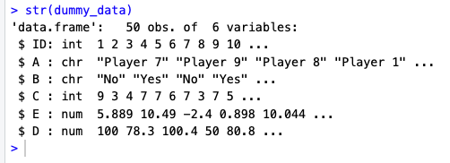
In R, you can type the str function to get a quick overview of the different types of data in your dataset.
In the figure above, we can see that the variable [A] is a character, while the variable [C] is an integer.
There are six basic types of data that R recognises. By clearly defining (and understanding) which type of data each variable holds, you will find it much easier to work with the data later on.
Numeric
Numeric data types are used in R to represent real numbers, including integers and decimals.
Examples include 42, -7, 3.14, 0.001.
The as.numeric() command can be used to convert a variable into the numeric type.
Integer
Integers are a subtype of the numeric data type, specifically used in R to represent whole numbers without decimals.
Examples include 5L, -3L (the ‘L’ suffix indicates that the number is an integer).
Character
Character data types are used in R to represent text data, including individual characters, strings, and words.
They are always enclosed in double or single quotes (you can use either). Examples include “hello”, ‘R programming’.
Logical
Logical data types represent Boolean (true/false) values.
They are used in R to make comparisons and to perform logical operations.
As noted above, logical values must be entered in capitals, for example TRUE, FALSE.
Factors
Factors represent categorical data as integer codes (e.g., 1, 2), as well as a corresponding list of unique character labels that tell R what each code represents (e.g., 1=Male, 2=Female).
They are particularly useful for storing and analyzing nominal and ordinal data. Examples include Gender (Male, Female), Age Group (Child, Teen, Adult).
In sport data, we will often use factors to define team names, which country the athlete was from, whether a game was home or away, or which season the data was collected. Factors allow us to easily compare different groups or categories.
Remember that a factor can also represent the same individual or team on multiple occasions, rather than refer to separate people or teams.
Date and Date-time
The ‘Date’ type in R represents dates in the format YYYY-MM-DD. This avoids confusion between DD/MM/YYYY and MM/DD/YYYY!
The Date-time type also represents dates, but includes time information (hours, minutes, seconds) as well.
This data type is useful for handling time series data and date-based calculations. Examples include “2021-09-01”, “2021-09-01 12:34:56”.
In the module ‘Research Methods for Sport Data Analytics’ in Semester 2, we’ll cover the use of dates and times in R in much more detail as part of a section on time-series analysis (TSA).
4.4 Vectors and Basic Vector Operations
The concept of a vector is fundamental to data analytics. Basically, a vector is an ordered collection of elements.
In R, all elements in a vector must be the same data type (i.e., the elements can only be one of the types discussed above).
Vectors are the ‘building blocks’ of more complex data structures such as dataframes, which we’ll cover shortly.
When you have data stored in a vector, you can perform a number of different operations on that vector (for example, by combining it with other vectors).
Creating vectors
We can use the c() function to create a vector by combining elements.
Important
Remember, all elements in a vector have to be of the same type.
# create a numeric vector with five elementsnumeric_vector <-c(1, 2, 3, 4, 5)# create a character vector with three elementscharacter_vector <-c("playerOne", "playerTwo", "playerThree")# create a logical vector with three elementslogical_vector <-c(TRUE, FALSE, TRUE)
Accessing vector elements
We can use square brackets ‘[ ]’ with an index or a range to access specific elements in a vector. For example, you may wish to extract the first ten elements in a vector.
Note
R uses 1-based indexing (or numbering), so the first element in the vector has an index of 1. Some other programming languages use 0-based indexing, where the first element has an index of 0.
second_element <- numeric_vector[2] # gets the second element in the vector numeric_vectorfirst_three_elements <- character_vector[1:3]last_element <- logical_vector[length(logical_vector)]# print results to consoleprint(second_element)
[1] 2
print(first_three_elements)
[1] "playerOne" "playerTwo" "playerThree"
print(last_element)
[1] TRUE
Modifying vectors
In addition to extracting parts of a vector, we can also add or update elements by assigning values using indexing:
numeric_vector[2] <-42# puts the value 42 into the second element of the vectorcharacter_vector <-c(character_vector, "orange")logical_vector[length(logical_vector)] <-FALSE
Vector operations
We can also perform element-wise arithmetic and logical operations on vectors:
a <-c(1, 2, 3)b <-c(4, 5, 6)sum_vector <- a + bprint(sum_vector)
[1] 5 7 9
product_vector <- a * bprint(product_vector)
[1] 4 10 18
Vector functions
We can apply functions to vectors to perform various operations: