| A1 | A2 | A3 | A4 |
|---|---|---|---|
| 3.8 | 5.2 | 6.7 | 4.1 |
| 4.6 | 3.9 | 5.3 | 3.7 |
| 8.1 | 8.6 | 2.6 | 4.6 |
| 5.1 | 6.0 | 7.5 | 2.3 |
| 5.2 | 1.0 | 6.0 | 9.2 |
| 8.4 | 6.3 | 4.5 | 7.3 |
Canonical Correlation Analysis
Week 4 2025, B1705
Introduction
- This presentation demonstrates Canonical Correlation Analysis (CCA) as a step-by-step.
- We’ll use two datasets, A and B, each containing four variables.
| B1 | B2 | B3 | B4 |
|---|---|---|---|
| 6.6 | 4.3 | 5.4 | 8.2 |
| 6.0 | 3.8 | 3.6 | 8.0 |
| 5.9 | 6.6 | 6.4 | 7.1 |
| 8.6 | 7.0 | 5.7 | 6.5 |
| 5.5 | 6.1 | 5.9 | 4.7 |
| 9.0 | 7.9 | 6.9 | 8.6 |
Process
Step One: Centering the Data
First, we center the data…
- We subtract the mean from each variable.
- This makes our data easier to analyse by removing biases.
Centered data
| A1 | A2 | A3 | A4 |
|---|---|---|---|
| -1.6 | 1.0 | 1.0 | -0.7 |
| -0.8 | -0.3 | -0.4 | -1.1 |
| 2.7 | 4.4 | -3.1 | -0.2 |
| -0.3 | 1.8 | 1.8 | -2.5 |
| B1 | B2 | B3 | B4 |
|---|---|---|---|
| 0.3 | -1.7 | -0.7 | 1.3 |
| -0.3 | -2.2 | -2.5 | 1.1 |
| -0.4 | 0.6 | 0.3 | 0.2 |
| 2.3 | 1.0 | -0.4 | -0.4 |
Compute the Variance
Now, we compute the covariance
- Covariance tells us how variables change together.
- We calculate it for each dataset and also between them.
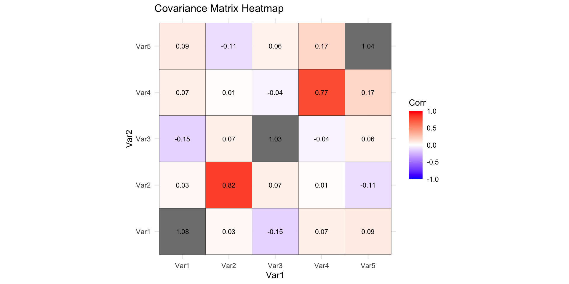
What is a Covariance Matrix?
A covariance matrix shows how different variables change together.
It helps us understand relationships between multiple variables in a dataset.
Interpreting a covariance matrix
- Positive values mean that when one variable increases, the other tends to increase too.
- Negative values mean that when one variable increases, the other tends to decrease.
- Zero values mean that the variables are not related.
Each element in the matrix represents the covariance between a pair of variables, and the diagonal values show the variance of each variable.
Visualisation of a covariance matrix
Compute Covariance Matrices
So we compute the covariance matrices…
| A1 | A2 | A3 | A4 | |
|---|---|---|---|---|
| A1 | 3.19 | 1.65 | -1.55 | 0.72 |
| A2 | 1.65 | 4.10 | -1.02 | -1.25 |
| A3 | -1.55 | -1.02 | 1.72 | -0.58 |
| A4 | 0.72 | -1.25 | -0.58 | 3.68 |
| B1 | B2 | B3 | B4 | |
|---|---|---|---|---|
| B1 | 2.38 | -0.63 | 0.56 | 1.16 |
| B2 | -0.63 | 5.25 | 0.15 | -1.90 |
| B3 | 0.56 | 0.15 | 1.36 | -0.37 |
| B4 | 1.16 | -1.90 | -0.37 | 3.60 |
Calculating the covariance matrix between A and B
A covariance matrix (S_AB) between two datasets (A and B) measures how the variables in A change in relation to the variables in B.
This is different from the covariance matrices for A and B individually, which measure relationships among variables within the same dataset
Each entry in the A_B matrix represents the covariance between one variable in A and one variable in B.
If A1 and B1 have a high positive covariance, it means that when A1 increases, B1 also increases.
If they have a negative covariance, then when A1 increases, B1 tends to decrease.
If the covariance is close to zero, there is little or no relationship between them.
| B1 | B2 | B3 | B4 | |
|---|---|---|---|---|
| A1 | 0.23 | 1.62 | 0.65 | -1.40 |
| A2 | 1.11 | -0.01 | 0.08 | 1.22 |
| A3 | 0.16 | -0.22 | -0.12 | -0.10 |
| A4 | 0.48 | 0.57 | 0.57 | -0.74 |
Invert Covariance Matrices
Now we invert the covariance matrices
- We need to adjust the relationships between variables so they are easier to compare.
- To do this, we invert the covariance matrices, which is like finding an opposite operation.
- Sometimes, the inversion doesn’t work because the matrix is too similar in its values.
- In that case, we use a generalised inverse, which is a way to still get useful results.
Computing the Inverse of Covariance Matrices
| A1 | A2 | A3 | A4 | |
|---|---|---|---|---|
| A1 | 0.65 | -0.19 | 0.43 | -0.13 |
| A2 | -0.19 | 0.42 | 0.14 | 0.20 |
| A3 | 0.43 | 0.14 | 1.10 | 0.14 |
| A4 | -0.13 | 0.20 | 0.14 | 0.39 |
| B1 | B2 | B3 | B4 | |
|---|---|---|---|---|
| B1 | 0.60 | 0.00 | -0.31 | -0.23 |
| B2 | 0.00 | 0.24 | 0.01 | 0.13 |
| B3 | -0.31 | 0.01 | 0.92 | 0.20 |
| B4 | -0.23 | 0.13 | 0.20 | 0.44 |
Compute Canonical Correlations
Now we compute the Canonical Correlations
- Canonical correlation finds the strongest link between the datasets.
- It shows how one set of variables relates to another.
Compute Canonical Correlation
| Canonical_Correlations |
|---|
| 0.8557506 |
| 0.6137227 |
| 0.1952885 |
| 0.1125263 |
What does this tell us?
Each number represents the strength of the relationship between a pair of transformed variables from datasets A and B.
The 1st canonical correlation (0.86) is the strongest relationship between a weighted combination of A’s variables and a weighted combination of B’s variables.
Since 0.86 is close to 1, this means there is a strong connection between the two datasets.
What does this tell us?
- The 2nd canonical correlation (0.61) is the second strongest relationship.
- While still moderate, it is not as strong as the first pair.
What does this tell us?
- The 3rd and 4th canonical correlations are much weaker than the first two.
- This suggests that the third pair of transformed variables shares little relationship.
Key Takeaways
- The first one or two pairs are important and meaningful.
- The last two correlations are very weak and likely not useful.
- The analysis tells us that the strongest link between the datasets is captured by the first two pairs.
Compute Canonical Weights
Now we compute the canonical weights
- Canonical weights (coefficients) show how much each variable contributes to the correlation.
- A high absolute weight means that variable plays a big role in defining the relationship.
- A low absolute weight means that variable contributes very little.
- Positive weights suggest a direct relationship, while negative weights indicate an inverse relationship. :::
Compute Canonical Weights
| A1 | -0.21 | 0.03 | -0.02 | 0.08 |
| A2 | 0.06 | -0.18 | -0.02 | 0.02 |
| A3 | -0.18 | -0.14 | 0.19 | 0.07 |
| A4 | -0.02 | -0.12 | 0.00 | -0.13 |
| B1 | -0.08 | -0.18 | 0.10 | 0.03 |
| B2 | -0.03 | -0.03 | -0.09 | 0.10 |
| B3 | -0.04 | 0.02 | -0.20 | -0.19 |
| B4 | 0.14 | -0.03 | -0.13 | 0.02 |
Notice that the canonical weights for A1 and A2 in the first canonical function are -0.21 and 0.06.
This suggests that A1 has an important but negative role in defining the first canonical correlation, and A2 has a less important, but positive, impact.
Interpretation
- The first canonical correlation is the strongest relationship between the two datasets.
- The canonical weights show how each variable contributes to the correlation.
- Higher values indicate greater influence.
- Note: interpretation always depends on context of the data!