match_results <- read.csv('https://www.dropbox.com/scl/fi/2j81rn7tp7gbbwwk6u0mj/match_results.csv?rlkey=ut91g3i8x2p0lhazqtrfmzcml&dl=1')

match_stats <- read.csv('https://www.dropbox.com/scl/fi/uniigratwo2gbtjw5s5t1/match_stats.csv?rlkey=gp23mruaeqrwtthbu8g0vqshf&dl=1')

team_info <- read.csv('https://www.dropbox.com/scl/fi/54emt59ezuvbas21oxqxf/team_info.csv?rlkey=2sumcav36njagatv1cts6nijk&dl=1')Using SQL in Sport Data Analytics
B1700, Week Eight
Introduction to SQL
What is SQL?
SQL stands for Structured Query Language. It has:
Grammar (syntax): defined rules for how statements must be written (e.g. SELECT column FROM table WHERE condition).
Vocabulary (keywords): reserved words with specific meaning (SELECT, FROM, WHERE, etc.).
Semantics: each statement has a clear, predictable effect (e.g. filtering rows, updating data, creating a table).
SQL is a declarative language
SQL is declarative, not procedural (R is procedural, as is Python)
- That means you describe what you want, not how to get it.
For example:
SELECT name, age FROM students WHERE age > 20;
We don’t tell the database how to find those students. We declare the result we want and the database engine figures out the best way to produce it.
SQL is Domain-Specific
SQL is designed for a specific domain: relational data.
It’s not a general-purpose language like Python or Java; instead, it’s built to:
Query data
Manipulate data
Define database structures
Control access and transactions
What is a SQL database?
A SQL database stores structured data in tables, with rows representing records and columns representing attributes. This is called a relational database.
SQL allows us to use the Structured Query Language (SQL) to extract, filter, join, and summarise data efficiently.
SQL databases are ideal for managing large, relational datasets, where different tables are linked by keys.
SQL - Key Commands
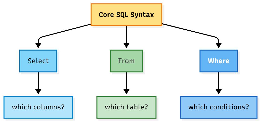
A very basic SQL query would be to select certain columns from a specific table where one or more conditions are met.
In plain English:
“select player_name and player_team from the table ‘player_data’, where player_gametime > 120.”
SQL code:
So in this SQL query:
SELECTchooses which columns to returnFROMindicates which table to queryWHEREfilters the rows
In R, the same thing could be achieved using the following code:
Grouping and Aggregating
SQL is often used to create new variables that are based on grouping and aggregating existing data.
In plain English:
“Look at the match_stats table and group the data by team. Then, for each team, calculate the average possession, and show the team name alongside that average.”
SQL code:
In this SQL query:
- We use
GROUP BYto summarise by group. - We use common functions:
AVG(),COUNT(),SUM()to create summaries.
Filtering Summaries: HAVING
In SQL, the command HAVING allows us to filter.
SQL code:
Sorting Results: ORDER BY
SQL code:
ORDER BYsorts results by column(s)- Add
DESCorASC
Joining Tables
JOINmerges rows with matching keys- Use
LEFT JOINto include unmatched rows from the left table
SQL code:
Common Table Expressions (CTEs)
- In SQL, we can use the
WITHcommand to structure multi-step queries cleanly:
Running SQL
Introduction
We can run SQL from many different environments (including R), depending on what we’re trying to do.
For future interviews/applications, it’s worth being at least vaguely familiar with the packages/platforms mentioned on the following slides.
Directly inside a database system
This is the most common way to run SQL.
You connect directly to a database management system (DBMS) such as:
PostgreSQL (using psql)
MySQL / MariaDB (using mysql)
SQLite (using sqlite3)
Microsoft SQL Server (using sqlcmd or SQL Server Management Studio)
Oracle Database (using sqlplus)
Each comes with a command-line tool or graphical interface where you can type and execute SQL statements directly.
Database management tools (GUI clients)
If you prefer a visual interface:
DBeaver (cross-platform, free)
TablePlus
DataGrip (JetBrains)
pgAdmin (for PostgreSQL)
HeidiSQL (for MySQL and others)
These let you connect to multiple databases, browse tables, and run SQL queries interactively.
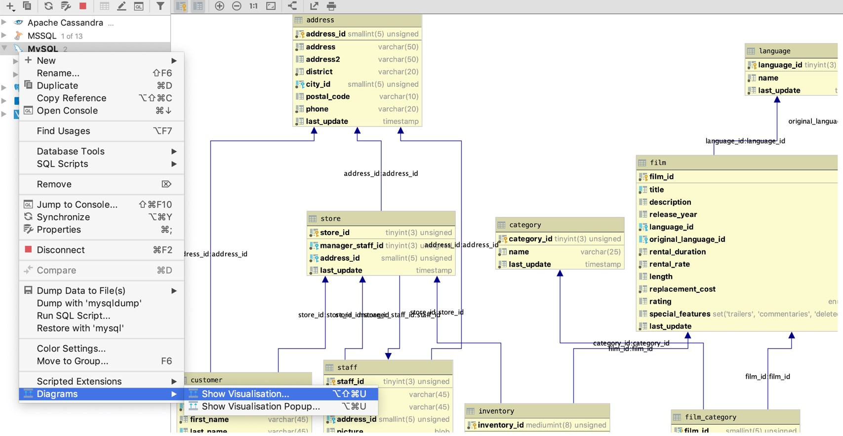
SQL in Datagrip
Within programming languages (including R)
You can run SQL from most major programming environments via connectors or libraries:
| Language | Common SQL interface |
|---|---|
| Python | sqlite3, sqlalchemy, pandas.read_sql() |
| Julia | SQLite.jl, ODBC.jl |
| Java | JDBC |
| C# / .NET | ADO.NET, Entity Framework |
| MATLAB | Database Toolbox |
| SAS / Stata / SPSS | PROC SQL or equivalent commands |
These languages send SQL statements to a database engine and retrieve results as data frames, tables, or lists.
From data analysis and BI tools
Many analytics and visualisation tools have built-in SQL query panels:
Power BI
Tableau
Google Data Studio / Looker Studio
Excel (via Power Query or Data Connections)
Apache Superset
Metabase
These tools use SQL under the hood to fetch and transform data before visualising it.
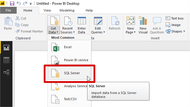
SQL in PowerBI
Inside notebooks and IDEs
Jupyter Notebooks with SQL extensions or ipython-sql
VS Code with SQL extensions
Azure Data Studio
RStudio supports both R and SQL chunks ({sql})
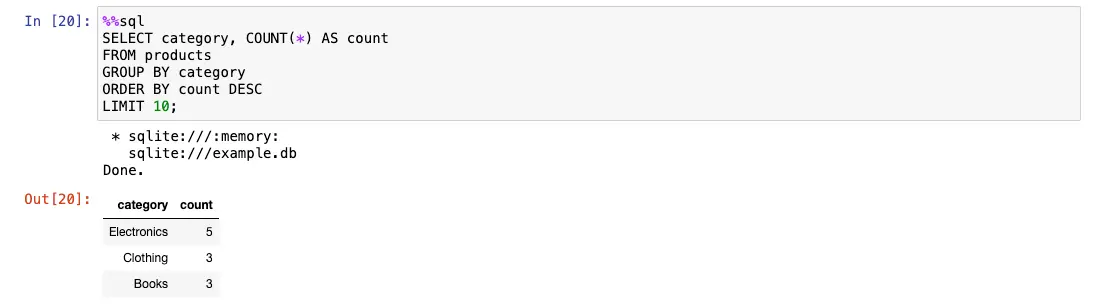
SQL in a Jupyter notebook
In the command line (PC) or terminal (Mac)
For small databases like SQLite, you can run SQL directly in the terminal:
sqlite3 mydata.db sqlite\> SELECT \* FROM customers;Using SQL in R
Basic steps
- Use
DBI::dbConnect()to connect to a database - Use
dbWriteTable()to load data - Query with
dbGetQuery(con, "your SQL here") - Always disconnect:
dbDisconnect(con)
Practical - Preparation
Loading the data
Start by downloading the following tables into your environment:
We’ll explore each of these to make sure we understand its contents.
Database connections
Before we can run any SQL queries in R using DBI, we need to create a connection to our SQLite database.
SQL engines operate on database files (not in-memory data frames like R), so we must tell R where our database is and how to communicate with it.
We will use the RSQLite package to connect to a database file called sportdata.sqlite.
Once connected, we can write SQL queries to extract and summarise data directly from the tables we’ve loaded into that file.
If the database file doesn’t already exist,
dbConnect()will create it.If your data is currently in R data frames (e.g., you’ve read the CSVs into
match_stats,team_info, andmatch_results), you’ll need to copy them into the SQLite database before querying.
Here’s how:
# Write R data frames to the connected SQLite database
# Assumes match_stats, team_info, and match_results are already loaded in your R environment.

dbWriteTable(con, "match_stats", match_stats, overwrite = TRUE)
dbWriteTable(con, "team_info", team_info, overwrite = TRUE)
dbWriteTable(con, "match_results", match_results, overwrite = TRUE)
This step creates actual tables inside your SQLite database. Once written, you can use SQL queries to access and analyse them just like in any database system.
We can check this:
Remember:
SQL engines don’t interact with R data frames directly. They require a connection to a database file (in our case,
sportdata.sqlite) where the tables are stored.Once connected, you can issue SQL commands using
dbGetQuery()just as you would inside a dedicated database tool.
Part 1: Exploring a Single Table
Working with a single table is a basic part of SQL.
Here, you’ll practise extracting and summarising data from the match_stats table using basic SQL commands like SELECT, WHERE, and GROUP BY.
These operations are essential for understanding how to retrieve meaningful summaries from raw data: in this case, match-by-match possession statistics across multiple teams.
Overview
Focus: match_stats table
Topics: SELECT, FROM, WHERE, ORDER BY, GROUP BY, HAVING
Core Task 1.1: To find the average possession by team:
In SQL, this would look like:
This will:
SELECT team: Returns one row per team.
AVG(possession) AS avg_possession: Computes a new variable which is the average of the possession column for each group, and labels it avg_possession.
FROM match_stats: Specifies the source table.
GROUP BY team: Tells SQL to group the data by team name so that AVG is calculated separately for each team.
We can implement this SQL command in R as:
# DBI implementation
library(DBI)
con <- dbConnect(RSQLite::SQLite(), "sportdata.sqlite")
dbGetQuery(con, "SELECT team, AVG(possession) AS avg_possession FROM match_stats GROUP BY team")
team avg_possession
1 Aberdeen 54.27391
2 Celtic 52.02188
3 Dundee United 52.07407
4 Hearts 57.83333
5 Hibs 52.60769
6 Rangers 54.74444Core Task 1.2 - Filter to show only teams with average possession over 55:
In SQL this would look like:
Part 2: Joining Tables
Combine data from two related tables to enrich your analysis.
Focus: match_stats + team_info
Key concept: INNER JOIN
Code
           team      city avg_possession
1      Aberdeen  Aberdeen       54.27391
2        Celtic   Glasgow       52.02188
3 Dundee United    Dundee       52.07407
4        Hearts Edinburgh       57.83333
5          Hibs Edinburgh       52.60769
6       Rangers   Glasgow       54.74444
Part 3: Multi-Table Summary (streamlined)
Bring together all three tables to produce a simple performance summary.
Focus: match_stats, match_results, team_info Key concepts: JOIN, GROUP BY, WHERE
Code
           team      city avg_possession total_goals
1      Aberdeen  Aberdeen       53.33333          27
2        Celtic   Glasgow       50.40769          30
3 Dundee United    Dundee       52.63684          56
4        Hearts Edinburgh       62.71429          19
5          Hibs Edinburgh       52.93846          38
6       Rangers   Glasgow       55.67143          33
Part 4: Open Practice & Recap
To practise and consolidate the essentials.
Suggested mini tasks:
Find teams with above-average possession.
Show top five teams by total goals (hint: ORDER BY).
Modify a join query to include one more variable.