rm(list=ls())

cat_data <- read.csv("https://www.dropbox.com/scl/fi/oxblp3vmk80s2203a91hf/categorical_data.csv?rlkey=50241qnzexvvmxgkj6gae5mlm&dl=1")7 Dealing with Categorical Data - Practical
7.1 Introduction
Following on from the pre-class reading, this tutorial introduces key concepts and techniques for working with categorical data in sport data analytics.
We’ll cover:
- encoding methods
- handling missing data
- visualising distributions
- building predictive models
7.2 Load Dataset
First, load the dataset as a dataframe called [cat_data]:
7.3 Defining Categorical Data
What is categorical data?
Categorical data are variables that fall into distinct groups or categories, such as “Sport”, “Gender”, and “League”.
They can either be nominal, with no inherent order, or ordinal, where the categories have a meaningful order.
Demonstration
Steps
- Examine the structure of the data.
- Identify categorical variables.
Code
# Check the structure of the dataset
str(cat_data)
'data.frame': 500 obs. of 8 variables:
$ PlayerID : int 1 2 3 4 5 6 7 8 9 10 ...
$ Sport : chr "Football" "Tennis" "Basketball" "Tennis" ...
$ Gender : chr "Female" "Female" "Female" "Female" ...
$ ExperienceLevel : chr "Intermediate" "Advanced" "Intermediate" "Beginner" ...
$ PerformanceScore: int 97 99 73 62 85 78 79 72 71 80 ...
$ AttendanceRate : chr "Moderate" "Moderate" "Moderate" "Low" ...
$ Region : chr "North" "West" "West" "East" ...
$ Outcome : chr "Win" "Lose" "Win" "Win" ...# Identify categorical variables
categorical_vars <- sapply(cat_data, is.character) | sapply(cat_data, is.factor)
cat("Categorical Variables:", names(cat_data)[categorical_vars])Categorical Variables: Sport Gender ExperienceLevel AttendanceRate Region OutcomeExercise
- Use
str()to review the structure of the dataset. - Review which variables are categorical, specifying whether they are nominal or ordinal.
7.4 Encoding Categorical Variables
Why encode categorical variables?
Machine learning algorithms often require numeric inputs, meaning we need to convert categorical data into numerical forms.
Encoding methods such as one-hot encoding and label encoding transform categories into numeric values that models can process.
Demonstration
Steps
- Review one-hot encoding.
- Apply one-hot encoding to [Sport] and [Gender].
- Review the new dataset structure.
Code
library(caret)Loading required package: ggplot2Loading required package: lattice# One-hot encoding
dummy_vars <- dummyVars("~ Sport + Gender", data = cat_data)
encoded_data <- predict(dummy_vars, newdata = cat_data)
# Combine encoded data with the original dataset
cat_data_encoded <- cbind(cat_data, encoded_data)
head(cat_data_encoded) PlayerID Sport Gender ExperienceLevel PerformanceScore AttendanceRate
1 1 Football Female Intermediate 97 Moderate
2 2 Tennis Female Advanced 99 Moderate
3 3 Basketball Female Intermediate 73 Moderate
4 4 Tennis Female Beginner 62 Low
5 5 Hockey Female Beginner 85 Moderate
6 6 Football Female Advanced 78 Low
Region Outcome SportBasketball SportFootball SportHockey SportTennis
1 North Win 0 1 0 0
2 West Lose 0 0 0 1
3 West Win 1 0 0 0
4 East Win 0 0 0 1
5 West Win 0 0 1 0
6 East Win 0 1 0 0
GenderFemale GenderMale
1 1 0
2 1 0
3 1 0
4 1 0
5 1 0
6 1 0Exercise
- Perform one-hot encoding for the variable [AttendanceRate].
- Review: what are the benefits and drawbacks of one-hot encoding?
Show solution
# Perform one-hot encoding on AttendanceRate
library(caret)
dummy_vars <- dummyVars("~ AttendanceRate", data = cat_data)
encoded_data <- predict(dummy_vars, newdata = cat_data)

# Add encoded columns to the dataset
cat_data_encoded <- cbind(cat_data, encoded_data)
head(cat_data_encoded)
PlayerID Sport Gender ExperienceLevel PerformanceScore AttendanceRate
1 1 Football Female Intermediate 97 Moderate
2 2 Tennis Female Advanced 99 Moderate
3 3 Basketball Female Intermediate 73 Moderate
4 4 Tennis Female Beginner 62 Low
5 5 Hockey Female Beginner 85 Moderate
6 6 Football Female Advanced 78 Low
Region Outcome AttendanceRateHigh AttendanceRateLow AttendanceRateModerate
1 North Win 0 0 1
2 West Lose 0 0 1
3 West Win 0 0 1
4 East Win 0 1 0
5 West Win 0 0 1
6 East Win 0 1 07.5 Handling Missing Categorical Data
Why do we need to handle missing data?
Like other forms of data, missing values in categorical variables can distort analyses and bias our models.
Common methods to address this include mode imputation (filling in missing values with the most frequent category) or creating a new “Missing” category.
Remember, since categorical data has no numerical meaning, we can’t use the median or mean for imputation.
Demonstration
Steps
- Check for missing values.
- Apply mode imputation to [AttendanceRate].
- Add a “Missing” category to [ExperienceLevel].
Code
# Check for missing values
colSums(is.na(cat_data))
PlayerID Sport Gender ExperienceLevel
0 0 0 30
PerformanceScore AttendanceRate Region Outcome
0 50 0 0 # Mode imputation for AttendanceRate
cat_data$AttendanceRate[is.na(cat_data$AttendanceRate)] <-
names(sort(table(cat_data$AttendanceRate), decreasing = TRUE))[1]
# Add a "Missing" category for ExperienceLevel
cat_data$ExperienceLevel[is.na(cat_data$ExperienceLevel)] <- "Missing"
table(cat_data$ExperienceLevel)
    Advanced     Beginner Intermediate      Missing
         141          144          185           30
Exercise
- Handle missing data in [Region] by creating a “Missing” category.
- Compare the proportion of missing values before and after handling.
Show solution
before <- sum(is.na(cat_data$Region))

# Handle missing values in Region by adding a "Missing" category
cat_data$Region[is.na(cat_data$Region)] <- "Missing"

# Compare proportions before and after handling

after <- sum(is.na(cat_data$Region))

cat("Missing values before handling:", before)
Missing values before handling: 0Show solution
cat("Missing values after handling:", after)Missing values after handling: 07.6 Exploratory Data Analysis (EDA) for Categorical Data
Why perform EDA?
EDA helps understand patterns, distributions, and relationships in the data.
In the context of categorical data, frequency tables and cross-tabulations are useful tools for understanding the prevalence of categories and their associations with other variables.
Demonstration
Steps
- Create frequency tables for categorical variables.
- Perform cross-tabulation to analyse relationships.
Code
# Frequency table for Sport
table(cat_data$Sport)
Basketball   Football     Hockey     Tennis
       148        209         48         95
# Cross-tabulation of Sport and Outcome
table(cat_data$Sport, cat_data$Outcome)
             Lose Win
  Basketball   14 134
  Football     10 199
  Hockey       13  35
  Tennis       17  78
Exercise
- Generate a frequency table for [Region].
- Analyse the relationship between [Gender] and [Outcome] using a cross-tabulation.
Show solution
# Frequency table for Region
freq_region <- table(cat_data$Region)
freq_region
 East North South  West
  123   127   125   125
Show solution
# Cross-tabulation of Gender and Outcome
cross_tab <- table(cat_data$Gender, cat_data$Outcome)
cross_tab
         Lose Win
  Female   23 219
  Male     31 227
7.7 Visualising Categorical Data
Why visualise categorical data?
Just like with continuous data, visualisations reveal insights into distributions and relationships within categorical data.
For example, bar charts and stacked bar charts can portray the distribution and relationships of categorical variables.
Demonstration
Steps
- Create a bar chart for [Sport].
- Add a stacked bar chart for [Sport] and [Outcome].
Code
library(ggplot2)

# Bar chart for Sport
ggplot(cat_data, aes(x = Sport)) +
  geom_bar(fill = "skyblue") +
  theme_minimal()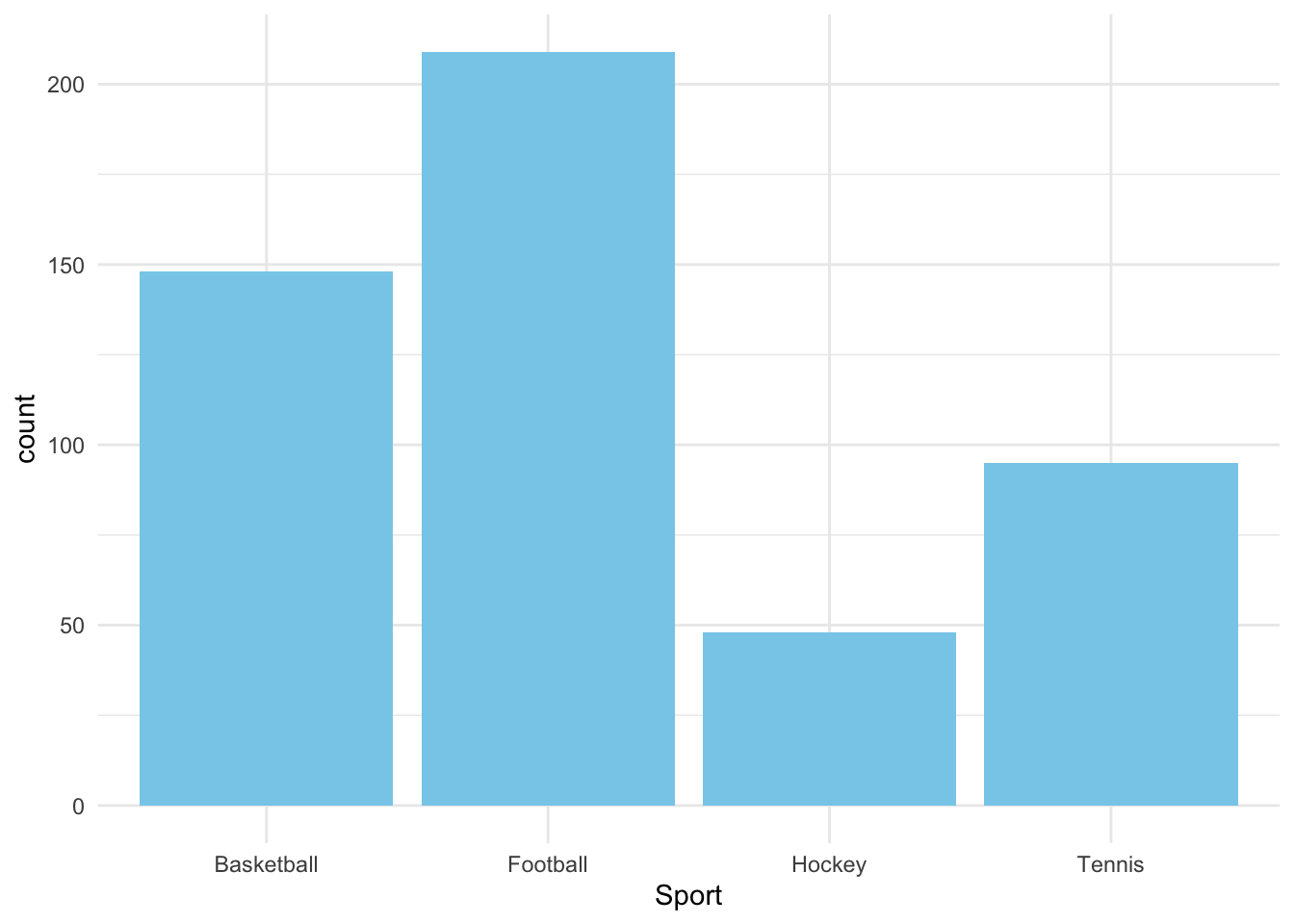
# Stacked bar chart
ggplot(cat_data, aes(x = Sport, fill = Outcome)) +
  geom_bar(position = "fill") +
  theme_minimal()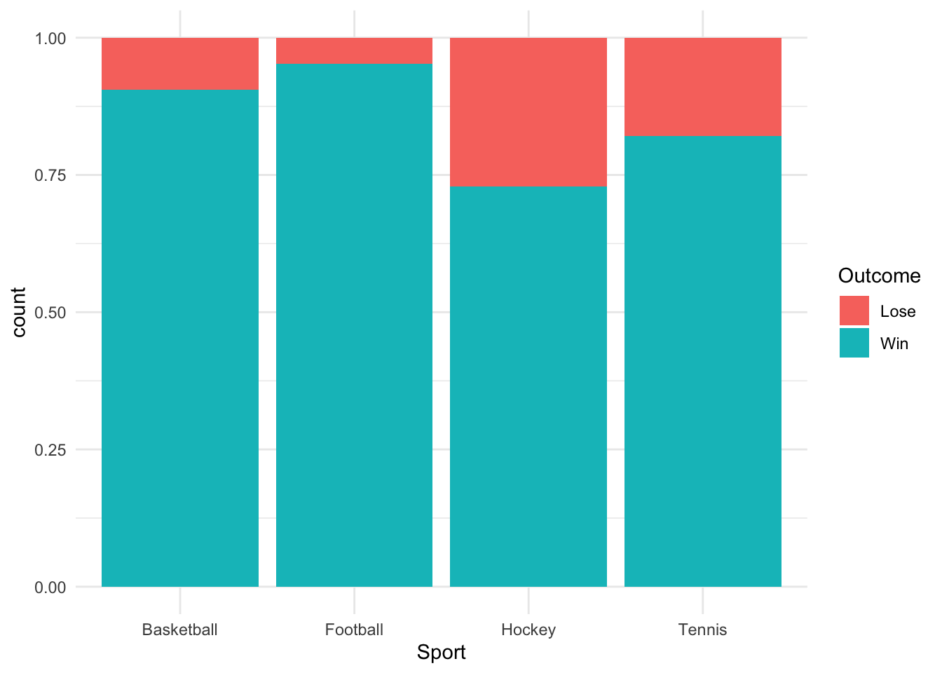
Exercise
- Create a bar chart for [AttendanceRate].
- Design a stacked bar chart for [Gender] and [Outcome].
#| code-fold: true
#| code-summary: Show solution


library(ggplot2)

# Bar chart for AttendanceRate
ggplot(cat_data, aes(x = AttendanceRate)) +
  geom_bar(fill = "blue") +
  theme_minimal()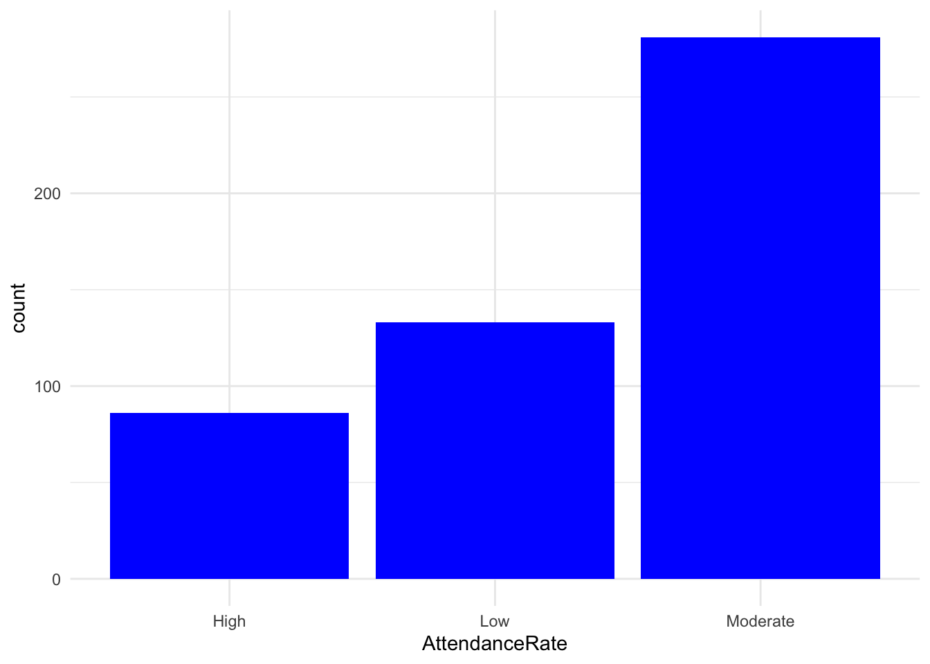
# Stacked bar chart for Gender and Outcome
ggplot(cat_data, aes(x = Gender, fill = Outcome)) +
  geom_bar(position = "fill") +
  theme_minimal()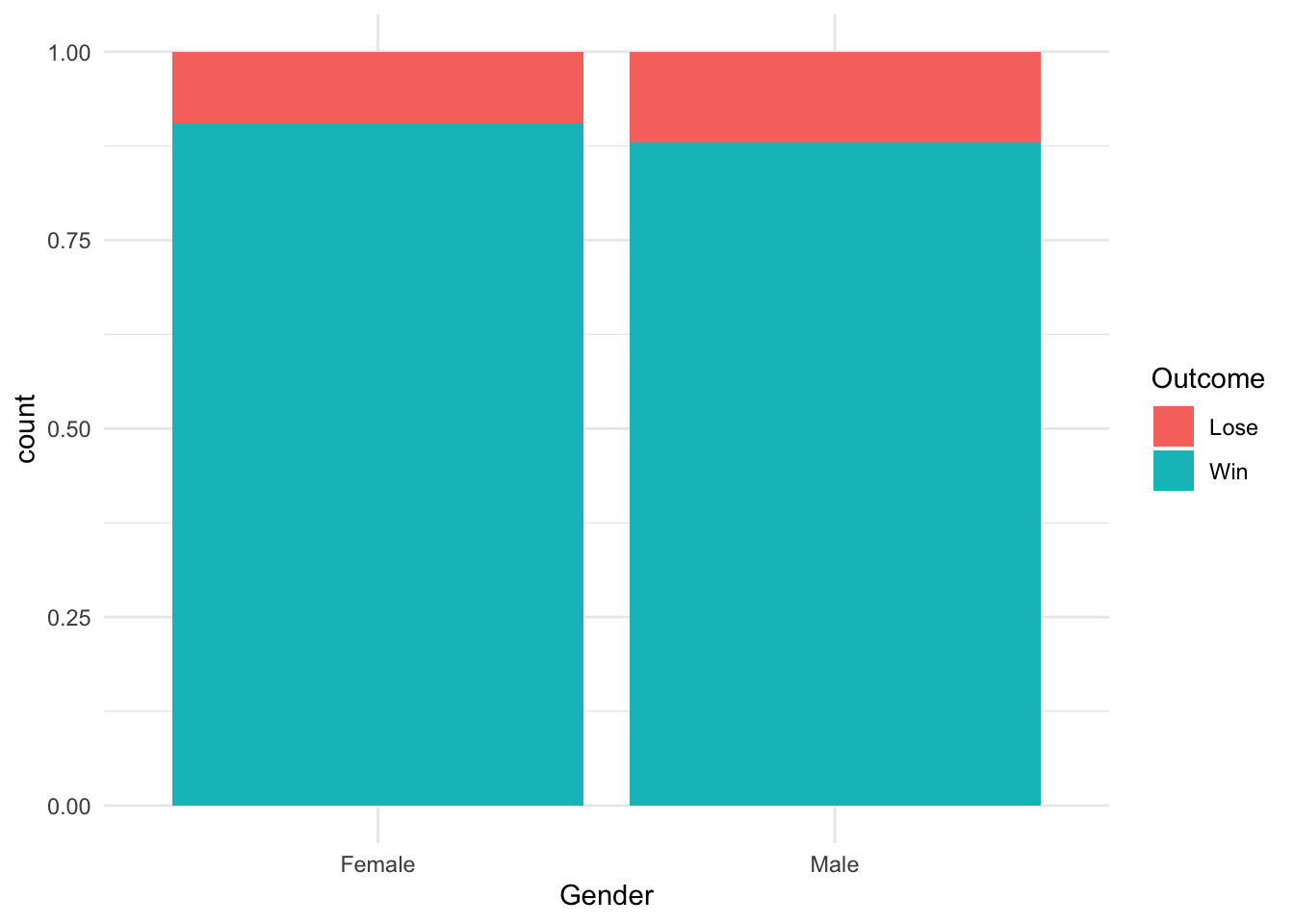
7.8 Statistical Methods for Categorical Data
Introduction
Statistical techniques such as logistic regression, Chi-square tests, and measures of association are designed to analyse relationships involving categorical variables:
- Logistic regression predicts binary outcomes (an outcome with only two levels). It performs a similar function to correlation.
- Chi-square tests assess the independence of categorical variables. It performs a similar function to tests of difference such as t-tests and ANOVA.
Demonstration
Steps
- Perform a Logistic Regression on [Outcome]: Predict categorical outcomes (lose or win) based on other variables.
- Perform a Chi-square Test: Assess relationships between [Sport] and [Outcome].
At the moment, we can’t run a logistic regression because the [Outcome] variable is not encoded as binary values (0 and 1), which are required for logistic regression. Logistic regression in R expects the dependent variable to be either numeric (0 and 1) or a factor with exactly two levels.
Code
# First, I need to convert [Outcome] to a factor with levels "Lose" (0) and "Win" (1)

cat_data$Outcome <- factor(cat_data$Outcome, levels = c("Lose", "Win"))

# Logistic regression
log_model <- glm(Outcome ~ Sport + Gender + AttendanceRate,
                 data = cat_data, family = "binomial")
summary(log_model)
Call:
glm(formula = Outcome ~ Sport + Gender + AttendanceRate, family = "binomial",
    data = cat_data)

Coefficients:
                       Estimate Std. Error z value Pr(>|z|)
(Intercept)              2.1516     0.4418   4.870 1.12e-06 ***
SportFootball            0.7165     0.4299   1.667  0.09556 .
SportHockey             -1.2651     0.4311  -2.935  0.00334 **
SportTennis             -0.7262     0.3895  -1.864  0.06227 .
GenderMale              -0.2263     0.3002  -0.754  0.45102
AttendanceRateLow        0.5155     0.4561   1.130  0.25846
AttendanceRateModerate   0.1936     0.3766   0.514  0.60716
---
Signif. codes:  0 '***' 0.001 '**' 0.01 '*' 0.05 '.' 0.1 ' ' 1

(Dispersion parameter for binomial family taken to be 1)

    Null deviance: 342.31  on 499  degrees of freedom
Residual deviance: 316.44  on 493  degrees of freedom
AIC: 330.44

Number of Fisher Scoring iterations: 5
# Chi-square test
chisq.test(table(cat_data$Sport, cat_data$Outcome))
    Pearson's Chi-squared test

data:  table(cat_data$Sport, cat_data$Outcome)
X-squared = 26.301, df = 3, p-value = 8.249e-06
Exercise
- Run logistic regression using [Region] as a predictor and [Outcome] as the outcome variable.
- Perform a Chi-square test to evaluate differences for [Gender] on the outcome [AttendanceRate].
Show solution
# Logistic regression for Region and Outcome
log_model <- glm(Outcome ~ Region, data = cat_data, family = "binomial")
summary(log_model)
Call:
glm(formula = Outcome ~ Region, family = "binomial", data = cat_data)

Coefficients:
            Estimate Std. Error z value Pr(>|z|)
(Intercept)   2.3206     0.3160   7.344 2.07e-13 ***
RegionNorth  -0.5196     0.4057  -1.281    0.200
RegionSouth   0.0177     0.4467   0.040    0.968
RegionWest   -0.2501     0.4246  -0.589    0.556
---
Signif. codes:  0 '***' 0.001 '**' 0.01 '*' 0.05 '.' 0.1 ' ' 1

(Dispersion parameter for binomial family taken to be 1)

    Null deviance: 342.31  on 499  degrees of freedom
Residual deviance: 339.90  on 496  degrees of freedom
AIC: 347.9

Number of Fisher Scoring iterations: 5
Show solution
# Chi-square test for Gender and AttendanceRate
chisq_test <- chisq.test(table(cat_data$Gender, cat_data$AttendanceRate))
chisq_test
    Pearson's Chi-squared test

data:  table(cat_data$Gender, cat_data$AttendanceRate)
X-squared = 0.28328, df = 2, p-value = 0.8679
7.9 Dealing with High Cardinality
Why manage high cardinality?
High cardinality occurs when categorical variables have many unique values.
Strategies like grouping infrequent categories can simplify variables, reduce noise, and improve our model interpretability without sacrificing significant information.
Demonstration
Steps
- Combine infrequent categories in [Region].
Code
cat_data$Region <- as.character(cat_data$Region)
cat_data$Region[cat_data$Region %in% c("North", "South")] <- "North-South"
table(cat_data$Region)
       East North-South        West
        123         252         125
Exercise
- Combine rare categories in the [Sport] variable.
- Review: how might high cardinality impact our modeling.
Show solution
# Combine rare categories in Sport
cat_data$Sport <- as.character(cat_data$Sport)
cat_data$Sport[cat_data$Sport == "Hockey"] <- "Other"
table(cat_data$Sport)
Basketball   Football      Other     Tennis
       148        209         48         95
7.10 Interaction Effects
Introduction
Interaction effects occur when the impact of one categorical variable depends on the level of another.
Including interaction terms in models can capture these relationships, enhancing predictive performance and providing insight into the interplay between variables.
Demonstration
Steps
- Explore interactions between categorical variables [Sport] and [Gender]
Code
# Interaction variable
cat_data$Sport_Gender <- interaction(cat_data$Sport, cat_data$Gender)
table(cat_data$Sport_Gender)
Basketball.Female   Football.Female      Other.Female     Tennis.Female
               66               109                21                46
  Basketball.Male     Football.Male        Other.Male       Tennis.Male
               82               100                27                49
Exercise
- Create an interaction variable for [Region] and [AttendanceRate].
- Analyse the new variable’s distribution.
Show solution
# Create an interaction variable for Region and AttendanceRate
cat_data$Region_Attendance <- interaction(cat_data$Region, cat_data$AttendanceRate)
table(cat_data$Region_Attendance)
           East.High     North-South.High            West.High
                  16                   45                   25
            East.Low      North-South.Low             West.Low
                  36                   70                   27
       East.Moderate North-South.Moderate        West.Moderate
                  71                  137                   73
7.11 Sparse Data
What is “sparse data”?
Sparse data refers to categories with very few observations, which can lead to instability in models and analyses.
We can combine sparse categories into broader groups or apply “regularisation” techniques can mitigate these challenges.
Demonstration
Steps
- Identify and resolve sparse categories.
Code
# Combine sparse categories in Gender
cat_data$Gender[cat_data$Gender == "Non-binary"] <- "Other"
table(cat_data$Gender)
Female   Male
   242    258
Exercise
- Identify sparse categories in [AttendanceRate] and resolve them.
Show solution
# Identify sparse categories in AttendanceRate
table(cat_data$AttendanceRate)
    High      Low Moderate
      86      133      281
Show solution
# Combine sparse categories
cat_data$AttendanceRate <- as.character(cat_data$AttendanceRate)
cat_data$AttendanceRate[cat_data$AttendanceRate == "Low"] <- "Other"
table(cat_data$AttendanceRate)
    High Moderate    Other
      86      281      133
7.12 Predictive Models Using Categorical Data Only
Introduction
Predictive models can use only categorical variables to predict outcomes.
Demonstration
Code
# Logistic regression with categorical variables
cat_model <- glm(Outcome ~ Sport + Gender + Region, data = cat_data, family = "binomial")
summary(cat_model)
Call:
glm(formula = Outcome ~ Sport + Gender + Region, family = "binomial",
    data = cat_data)

Coefficients:
                  Estimate Std. Error z value Pr(>|z|)
(Intercept)         2.5212     0.4385   5.750 8.94e-09 ***
SportFootball       0.7120     0.4297   1.657  0.09751 .
SportOther         -1.2544     0.4313  -2.908  0.00364 **
SportTennis        -0.7477     0.3887  -1.924  0.05440 .
GenderMale         -0.2116     0.2994  -0.707  0.47969
RegionNorth-South  -0.1971     0.3826  -0.515  0.60642
RegionWest         -0.1515     0.4374  -0.346  0.72917
---
Signif. codes:  0 '***' 0.001 '**' 0.01 '*' 0.05 '.' 0.1 ' ' 1

(Dispersion parameter for binomial family taken to be 1)

    Null deviance: 342.31  on 499  degrees of freedom
Residual deviance: 317.53  on 493  degrees of freedom
AIC: 331.53

Number of Fisher Scoring iterations: 5
7.13 Predictive Models Using Mixed Data
Introduction
We can also combine categorical and continuous variables in predictive models to enhance their explanatory and predictive power.
Demonstration
# Logistic regression with mixed variables
mixed_model <- glm(Outcome ~ Sport + Gender + PerformanceScore,
                   data = cat_data, family = "binomial")
summary(mixed_model)
Call:
glm(formula = Outcome ~ Sport + Gender + PerformanceScore, family = "binomial",
    data = cat_data)

Coefficients:
                 Estimate Std. Error z value Pr(>|z|)
(Intercept)       0.66488    0.84272   0.789  0.43013
SportFootball     0.73323    0.43097   1.701  0.08888 .
SportOther       -1.35516    0.43596  -3.108  0.00188 **
SportTennis      -0.71933    0.39130  -1.838  0.06602 .
GenderMale       -0.14581    0.30287  -0.481  0.63022
PerformanceScore  0.02290    0.01057   2.166  0.03030 *
---
Signif. codes:  0 '***' 0.001 '**' 0.01 '*' 0.05 '.' 0.1 ' ' 1

(Dispersion parameter for binomial family taken to be 1)

    Null deviance: 342.31  on 499  degrees of freedom
Residual deviance: 312.97  on 494  degrees of freedom
AIC: 324.97

Number of Fisher Scoring iterations: 5