4  Regression Analysis - Practical

This practical develops content from the previous section on Regression Analysis.

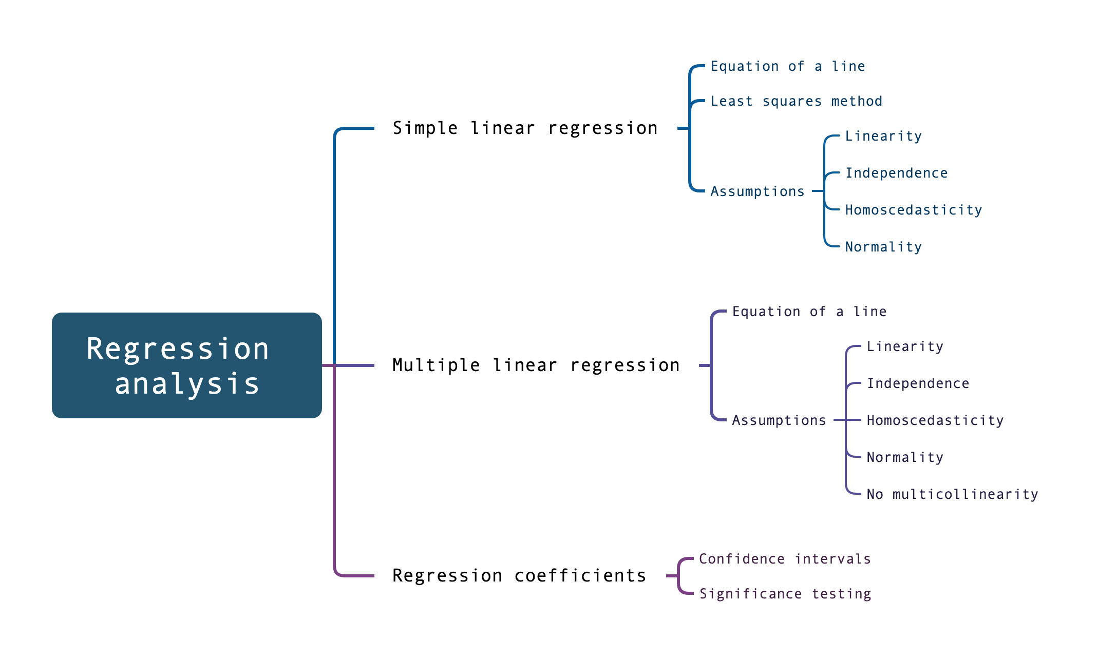
Objectives

• To gain confidence in conducting simple and multiple linear regression analysis using R.

• To gain practice in interpreting the output of regression models.

4.1 Assumptions

Regression models, like all statistical techniques, make some assumptions about the data that we ‘feed into’ them. Failing to meet these assumptions can fatally impact on the model’s predictive power.

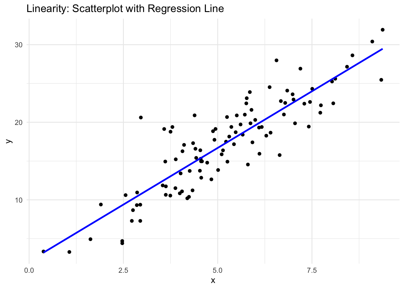
Linearity

Linear regression assumes that the effect of each predictor on the outcome is additive and linear. In other words, the combined effect of all predictors on the outcome is the sum of their individual effects.

\(y=β0​+β1​x1​+β2​x2​+⋯+βk​xk​+ϵ\)

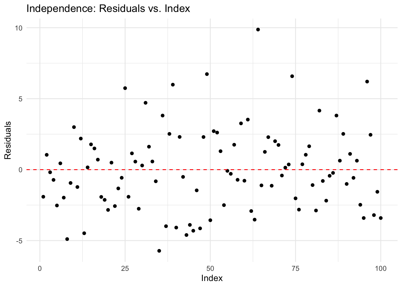
Independence

This means there is no autocorrelation. ‘Autocorrelation’ refers to the correlation of a time series with its own past and future values. It measures how well the current value of a variable is related to its previous values.

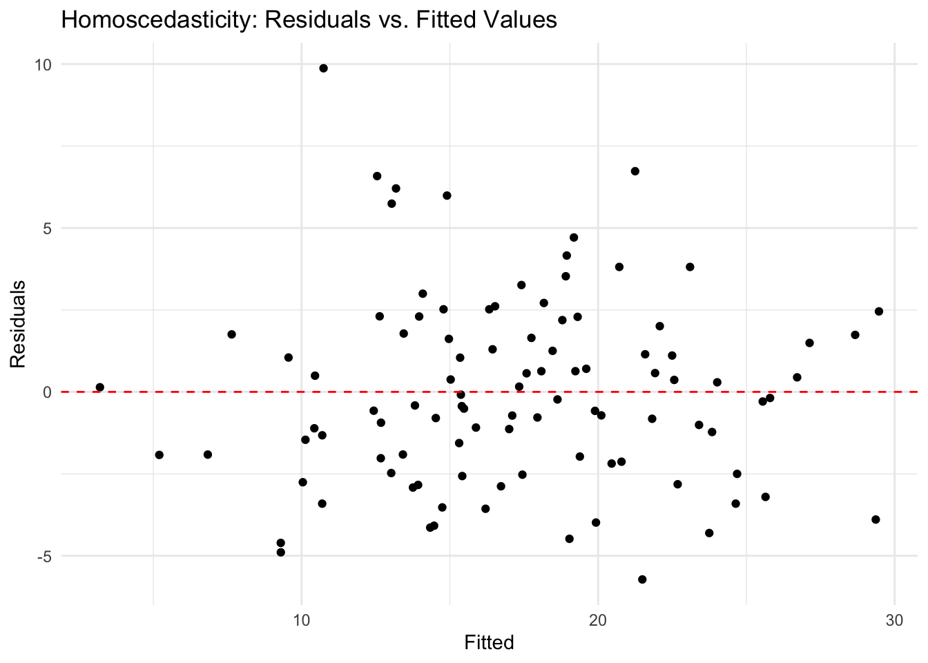
Homoscedasticity

Homoscedasticity means the spread of residuals is uniform, regardless of the values of the predictors or fitted values.

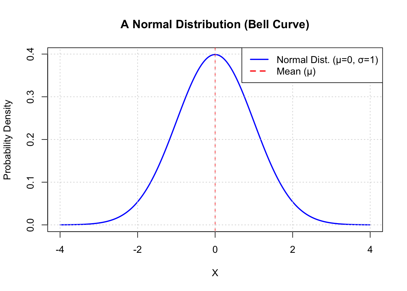
Normality

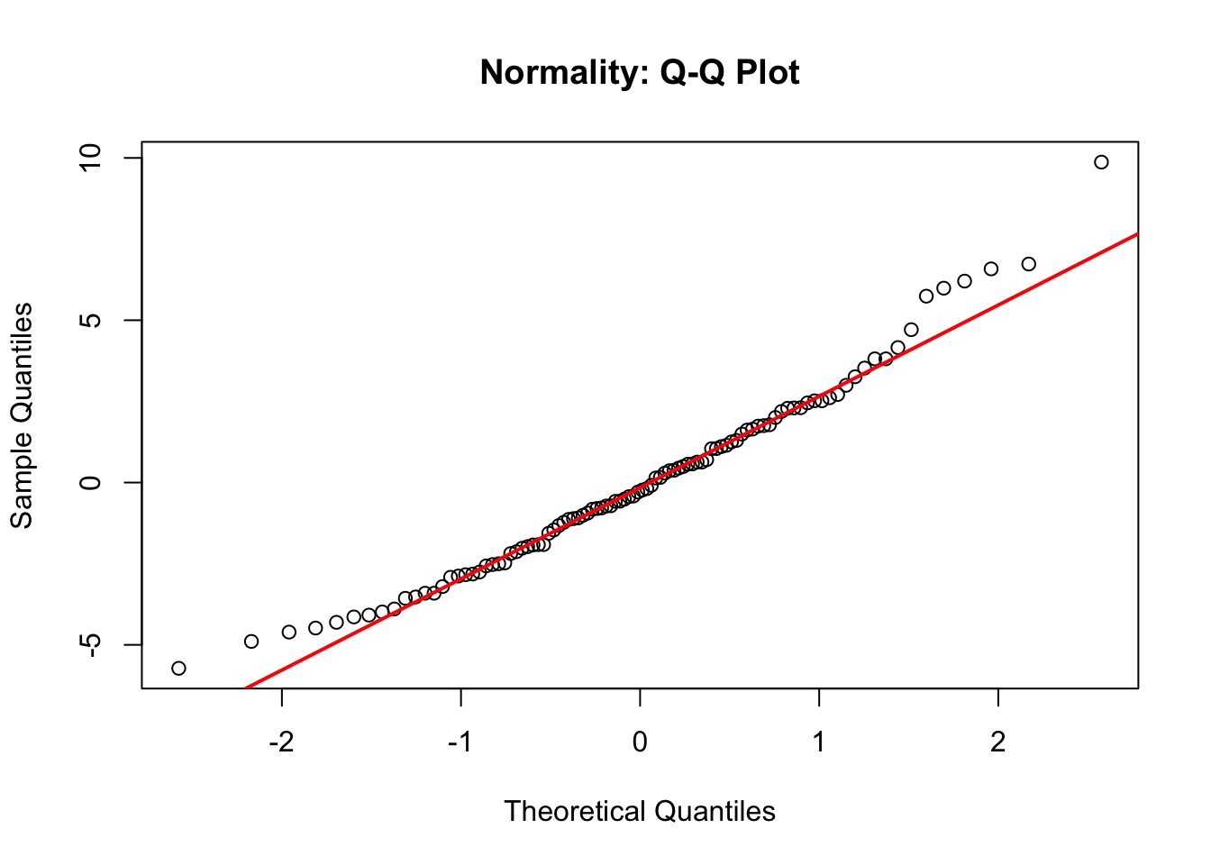
The data follows a normal distribution (a Gaussian distribution). A normal distribution is a bell-shaped curve that is symmetric about its mean, where most of the data points cluster around the central value and taper off equally on both sides.

This can be explored using a Q-Q plot (Quantile-Quantile). A Q-Q plot compares the distribution of the actual dataset to a ‘theoretical’ distribution, which is perfectly normal:

4.2 Simple linear regression: demonstration

Step 1: Data inspection

First, we’ll load a dataset. For this example, we’ll use the built-in mtcars dataset in R.

Show code to load datset

# Load the dataset
data(mtcars)

Step 2: Visualisation

Now, it’s helpful to visualise the data to understand the relationship between variables.

For instance, we can plot mpg (miles per gallon) against wt (weight of the car).

Show code to visualise data

# Load ggplot2
library(ggplot2)

# Create a scatter plot of mpg vs wt
ggplot(mtcars, aes(x = wt, y = mpg)) + 
    geom_point() +
    ggtitle("Scatter plot of MPG vs Car Weight") +
    xlab("Car Weight") +
    ylab("Miles per Gallon")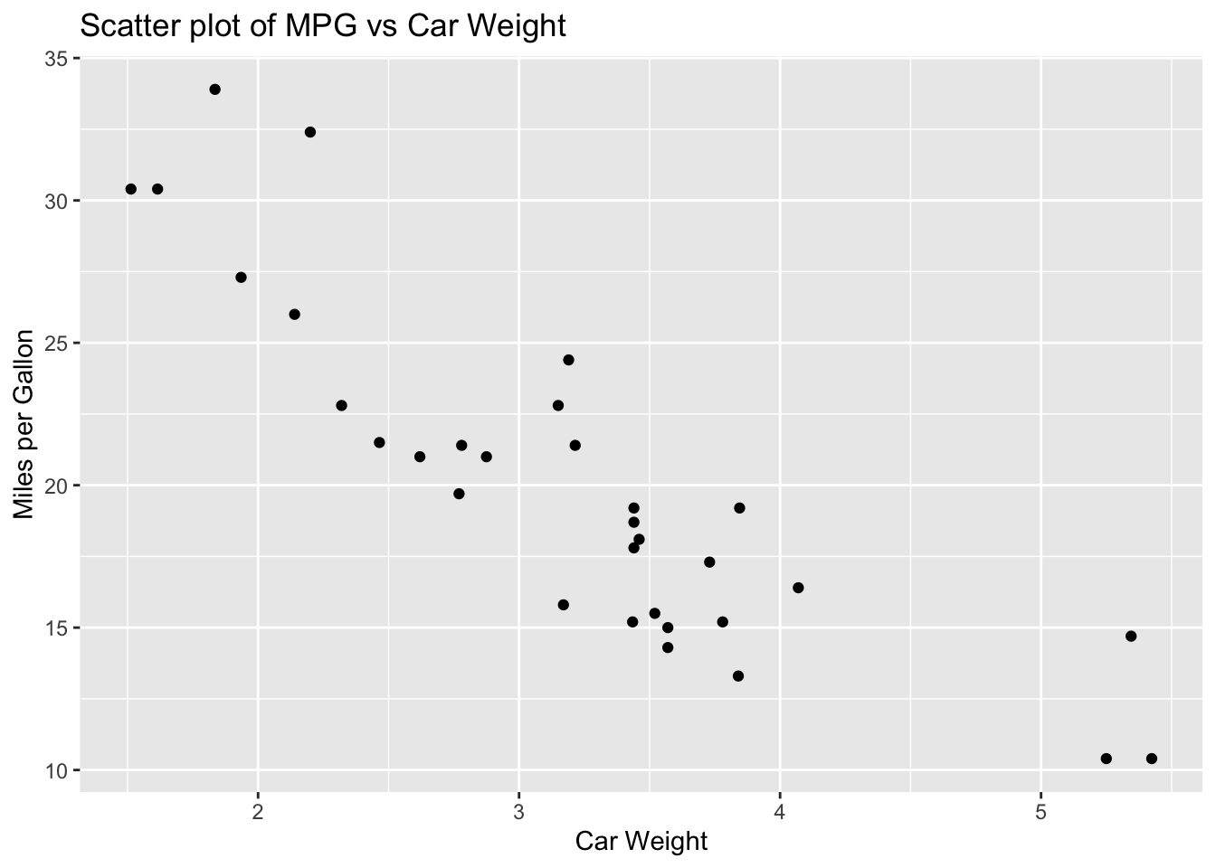

This plot helps us see if there’s a linear relationship between car weight and fuel efficiency. From the looks of it, it seems that miles per gallon decreases as car weight increases.

Step 3: Model fitting

To explore this relationship further, we’ll fit a simple linear regression model using the lm() function. In this example, the model specifies that we wish to examine the effect of weight [wt] on [mpg] (miles per gallon).

Show code

# Fit a linear model
model <- lm(mpg ~ wt, data = mtcars)

# View the model summary
summary(model)

Call:
lm(formula = mpg ~ wt, data = mtcars)

Residuals:
    Min      1Q  Median      3Q     Max 
-4.5432 -2.3647 -0.1252  1.4096  6.8727 

Coefficients:
            Estimate Std. Error t value Pr(>|t|)    
(Intercept)  37.2851     1.8776  19.858  < 2e-16 ***
wt           -5.3445     0.5591  -9.559 1.29e-10 ***
---
Signif. codes:  0 '***' 0.001 '**' 0.01 '*' 0.05 '.' 0.1 ' ' 1

Residual standard error: 3.046 on 30 degrees of freedom
Multiple R-squared:  0.7528,    Adjusted R-squared:  0.7446 
F-statistic: 91.38 on 1 and 30 DF,  p-value: 1.294e-10

Step 4: Output interpretation

The output from summary(model) provides several pieces of information.

• In the ‘Coefficients’ section, we’re provided with estimates for the intercept and slope. For each, you’ll see an estimate, standard error, t-value, and p-value.

• Towards the bottom, you will see ‘R-squared’. This indicates the proportion of variance in the dependent variable mpg that’s explained by the independent variable wt.

• You will also see p-values. The model tests the hypothesis that each coefficient is different from zero (no effect). A low p-value (< 0.05) suggests that the variable is significant in explaining mpg.

In our example, we could start by looking at the coefficient of wt: it’s negative and significant, suggesting that heavier cars tend to have lower fuel efficiency.

Turning to R-squared, this value is high (closer to 1). This indicates that our model explains a large portion of the variability in mpg.

Here’s a representation of the model, with the regression line in blue. This can be helpful in interpreting model output.

Show code

# Load library
library(ggplot2)

# Using the mtcars dataset
data(mtcars)

# Create a scatter plot of mpg vs wt with added regression line
ggplot(mtcars, aes(x = wt, y = mpg)) + 
    geom_point() + 
    geom_smooth(method = "lm", col = "blue") +
    ggtitle("Scatter Plot of MPG vs Car Weight with Regression Line") +
    xlab("Car Weight (1000 lbs)") +
    ylab("Miles per Gallon")

`geom_smooth()` using formula = 'y ~ x'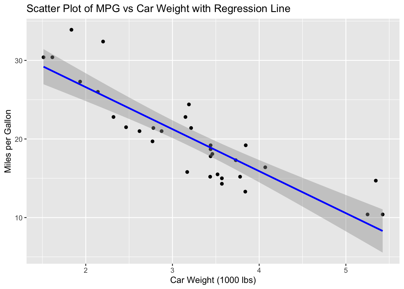

4.3 Simple linear regression: practice

Complete the following steps on the dataset available here:

Show code

df <- read.csv('https://www.dropbox.com/scl/fi/28mws7intbsetmkl7y885/17_01_dataset.csv?rlkey=en9hg7xbwcl169v8418qz48h2&dl=1')

1. Using a scatterplot, examine the relationship between Goals and Assists. Do you think there is a relationship between these two variables?
2. Check your assumption using simple linear regression.
3. Create a plot that summarises the relationship of these variables (scatterplot with regression line).
4. Using the format provided in the previous section, report the results of your analysis.
5. Repeat steps 2-5 for PIM and IceTime.
6. Repeat steps 2-5 for Goals and IceTime.

4.4 Multiple linear regression: demonstration

As noted previously, multiple linear regression expands the concept of simple linear regression to include more than one predictor (independent) variable in the model.

This makes things more complicated and requires us to consider issues such as multicollinearity.

What is multicollinearity?

Multicollinearity in statistical modeling, particularly in multiple linear regression, refers to a situation where two or more predictor variables are highly correlated with each other.

Step 1: Adding variables

We’ll continue using the mtcars dataset, which is included in R. In addition to wt (car weight), we’ll also consider hp (horsepower) and qsec (1/4 mile time) as predictors for mpg (miles per gallon).

Show code

# Load the dataset
data(mtcars)

Step 2: Model fitting

As we did in simple linear regression, we can use the lm() function to fit a multiple linear regression model.

Show code for the regression model

# Fit a multiple linear regression model
model <- lm(mpg ~ wt + hp + qsec, data = mtcars)

# View the model summary
summary(model)

Call:
lm(formula = mpg ~ wt + hp + qsec, data = mtcars)

Residuals:
    Min      1Q  Median      3Q     Max 
-3.8591 -1.6418 -0.4636  1.1940  5.6092 

Coefficients:
            Estimate Std. Error t value Pr(>|t|)    
(Intercept) 27.61053    8.41993   3.279  0.00278 ** 
wt          -4.35880    0.75270  -5.791 3.22e-06 ***
hp          -0.01782    0.01498  -1.190  0.24418    
qsec         0.51083    0.43922   1.163  0.25463    
---
Signif. codes:  0 '***' 0.001 '**' 0.01 '*' 0.05 '.' 0.1 ' ' 1

Residual standard error: 2.578 on 28 degrees of freedom
Multiple R-squared:  0.8348,    Adjusted R-squared:  0.8171 
F-statistic: 47.15 on 3 and 28 DF,  p-value: 4.506e-11

In this example, we have created a model that assumes that mpg is influenced by three different predictor variables wt, hp and qsec.

Step 3: Multicollinearity check

Multicollinearity refers to a situation in which two or more explanatory variables in a multiple regression model are highly linearly related. We use the vif() function from the car package to check for this.

First, we load the car package. Then we check for multicollinearity using the vif function.

Show code to run VIF on our model

# Load the car package, which lets us calculate VIF
library(car)

Loading required package: carData

Show code to run VIF on our model

# Then, check for multicollinearity
vif(model)

      wt       hp     qsec 
2.530443 4.921956 2.873804 

Note: Values of VIF (Variance Inflation Factor) greater than 5 or 10 indicate a problematic amount of collinearity.

Step 4: Output interpretation

The output of summary(model) contains several important pieces of information:

Coefficients

These are the estimated values of the regression coefficients for each predictor. A p-value Pr(\>\|t\|) is provided to test the null hypothesis that the coefficient is equal to zero.

From the model summary, we can see that wt is significantly associated with mpg, but hp and qsec are not.

The estimated value for wt is negative, indicating that our outcome variable mpg decreases as wt increases.

The coefficients indicate the expected change in mpg for a one-unit increase in the predictor, holding other predictors constant.

Multiple R-squared

This is the proportion of variance in the dependent variable that is predictable from the independent variables. It ranges from 0 to 1.

A high R-squared value suggests a good fit, but should be considered along with the adjusted R-squared.

In our model, R-squared is high, suggesting our model is a good ‘fit’ for the data.

Adjusted R-squared

This is a modified version of R-squared adjusted for the number of predictors in the model. It is generally considered a more accurate measure of the goodness of fit, especially for multiple regression. Adjusted R-squared adjusts for the number of predictors, so it’s a better measure of fit for multiple regression.

4.5 Multiple linear regression: practice

Complete the following steps:

1. Download the data file:

Show code to load dataset

df <- read.csv('https://www.dropbox.com/scl/fi/4eb55qzffd3cdnrpl5h0i/mreg_01.csv?rlkey=zddodcpd6df5xfwivkyhefett&dl=1')

1. Conduct a multiple linear regression in which the influence of predictors (IVs) on an outcome variable score (DV) is explored.

2. Using the format provided earlier, report the results of your analysis.

4.6 More on regression coefficients: demonstration

in the final part of this practical we’ll review the interpretation of regression coefficients in R, covering the extraction of coefficients, standardisation of variables, and significance testing.

Dataset

We’ll use the mtcars dataset for this tutorial, focusing on predicting mpg (miles per gallon) from wt (weight) and hp (horsepower).

Load the dataset

# Load the dataset
data(mtcars)

Coefficient extraction

First, we’ll fit a linear regression model and extract the unstandardised coefficients.

Fit the model

# Fit the model
model <- lm(mpg ~ wt + hp, data = mtcars)

# Extracting unstandardized coefficients
coefficients <- coef(model)
print(coefficients)

(Intercept)          wt          hp 
37.22727012 -3.87783074 -0.03177295 

The intercept is the estimated average value of mpg when wt and hp are both 0.

The coefficients for wt and hp represent the change in mpg for a one-unit increase in wt or hp, keeping the other constant.

Standardisation

To interpret the coefficients in terms of standard deviations, we need standardise the variables (so we’re comparing ‘like with like’).

Standardise variables

# Standardising the variables
mtcars$wt_std <- scale(mtcars$wt)
mtcars$hp_std <- scale(mtcars$hp)

# Fitting the model with standardised predictors
model_std <- lm(mpg ~ wt_std + hp_std, data = mtcars)

# Extracting standardized coefficients
coefficients_std <- coef(model_std)
print(coefficients_std)

(Intercept)      wt_std      hp_std 
  20.090625   -3.794292   -2.178444 

Now the coefficients represent the change in mpg for a one standard deviation increase in wt or hp.

Significance testing

We’ll look at the summary of our model to perform hypothesis tests on the coefficients.

View model

# Viewing the summary of the model
summary(model)

Call:
lm(formula = mpg ~ wt + hp, data = mtcars)

Residuals:
   Min     1Q Median     3Q    Max 
-3.941 -1.600 -0.182  1.050  5.854 

Coefficients:
            Estimate Std. Error t value Pr(>|t|)    
(Intercept) 37.22727    1.59879  23.285  < 2e-16 ***
wt          -3.87783    0.63273  -6.129 1.12e-06 ***
hp          -0.03177    0.00903  -3.519  0.00145 ** 
---
Signif. codes:  0 '***' 0.001 '**' 0.01 '*' 0.05 '.' 0.1 ' ' 1

Residual standard error: 2.593 on 29 degrees of freedom
Multiple R-squared:  0.8268,    Adjusted R-squared:  0.8148 
F-statistic: 69.21 on 2 and 29 DF,  p-value: 9.109e-12

Each coefficient’s t-value and Pr(\>\|t\|) (p-value) are used to test the null hypothesis that the coefficient is zero. A small p-value (< 0.05) suggests rejecting the null hypothesis, indicating a significant relationship.

The R-squared value suggests that ~ 83% of the variance in mpg is explained by our model.